zpk

Null-Polstellen-Verstärkungsmodell

Beschreibung

Verwenden Sie zpk, um reellwertige oder komplexwertige Null-Polstellen-Verstärkungsmodelle zu erstellen oder um dynamische Systemmodelle in die Form eines Null-Polstellen-Verstärkungsmodells zu konvertieren.

Null-Polstellen-Verstärkungsmodelle stellen Transferfunktionen in faktorisierter Form dar. Betrachten Sie in diesem Beispiel die folgende zeitkontinuierliche SISO-Transferfunktion:

$$G\left(s\right)=\frac{s^2-3s-4}{s^2+5s+6}$$

G(s) kann folgendermaßen in die Null-Polstellen-Verstärkungsform faktorisiert werden:

$$G\left(s\right)=\frac{\left(s+1\right)\left(s-4\right)}{\left(s+2\right)\left(s+3\right)}.$$

Eine allgemeinere Darstellung des SISO-Null-Polstellen-Verstärkungsmodells:

$$h\left(s\right)=k\frac{\left(s-z\left(1\right)\right)\left(s-z\left(2\right)\right)\dots \left(s-z\left(m\right)\right)}{\left(s-p\left(1\right)\right)\left(s-p\left(2\right)\right)\dots \left(s-p\left(n\right)\right)}$$

Hier sind z und p die Vektoren der reellwertigen oder komplexwertigen Nullstellen und Polstellen und k ist die reellwertige oder komplexwertige skalare Verstärkung. Bei MIMO-Modellen wird jeder E/A-Kanal durch eine derartige Transferfunktion h_ij(s) dargestellt.

Sie können ein Null-Polstellen-Verstärkungsmodellobjekt entweder durch direkte Angabe von Polstellen, Nullstellen und Verstärkungsfaktoren oder durch die Konvertierung eines anderen Modelltyps (wie einem Zustandsraummodell ss) in Null-Polstellen-Verstärkungsform erstellen.

Sie können zpk auch verwenden, um verallgemeinerte Zustandsraummodelle (genss) oder unsichere Zustandsraummodelle (uss (Robust Control Toolbox)) zu erstellen.

Erstellung

Syntax

sys = zpk(zeros,poles,gain)

sys = zpk(zeros,poles,gain,ts)

sys = zpk(zeros,poles,gain,ltiSys)

sys = zpk(m)

sys = zpk(___,PropertyName=Value)

sys = zpk(ltiSys)

sys = zpk(ltiSys,Name=Value)

sys = zpk(ltiSys,component)

s = zpk('s')

z = zpk('z',ts)

Beschreibung

Erstellen eines ZPK-Modells

sys = zpk(zeros,poles,gain) erstellt ein zeitkontinuierliches Null-Polstellen-Verstärkungsmodell aus zeros und poles (als Vektoren angegeben) und dem skalaren Wert von gain. Der Ausgang sys ist ein zpk-Modellobjekt, in dem die Modelldaten gespeichert sind. Setzen Sie für Systeme oder Nullstellen oder Polstellen zeros oder poles auf []. Diese zwei Eingänge müssen nicht die selbe Länge aufweisen und das Modell muss nicht ordnungsgemäß sein (d. h. einen Polstellen-Überschuss aufweisen).

sys = zpk(zeros,poles,gain,ts) erstellt ein zeitdiskretes Null-Polstellen-Verstärkungsmodell mit der Abtastzeit ts. Setzen Sie ts auf -1 oder [], um keine Abtastzeit anzugeben.

sys = zpk(zeros,poles,gain,ltiSys) erstellt ein Null-Polstellen-Verstärkungsmodell mit Eigenschaften, die vom dynamischen Systemmodell ltiSys geerbt wurden, einschließlich der Abtastzeit.

sys = zpk(m) erstellt ein Null-Polstellen-Verstärkungsmodell, das den statischen Verstärkungsfaktor m darstellt.

sys = zpk(___,PropertyName=Value) legt Eigenschaften des Null-Polstellen-Verstärkungsmodells fest, indem es ein oder mehrere Eigenschaftsname-Wert-Argumente zum Festlegen weiterer Modelleigenschaften verwendet. Diese Syntax funktioniert bei allen vorherigen Eingang-Argument-Kombinationen.

Konvertieren zu einem ZPK-Modell

sys = zpk(ltiSys) konvertiert das dynamische Systemmodell ltiSys in ein Null-Polstellen-Verstärkungsmodell.

sys = zpk(ltiSys,Name=Value) erhält eine verkürzte zpk-Darstellung des schwach besetzten Modells ltiSys durch Berechnung der Nullstellen und Polstellen auf der Grundlage eines oder mehrerer angegebener Name-Wert-Argumente. Da diese Methode Nullstellen für jedes Eingangs-Ausgangs-Paar berechnet, ist sie am besten für Modelle mit kleinen Eingangs-Ausgangs-Größen geeignet. (seit R2025a)

sys = zpk(ltiSys,component) konvertiert die angegebene Komponente component von ltiSys in die Form eines Null-Polstellen-Verstärkungsmodells. Verwenden Sie diese Syntax nur, wenn es sich bei ltiSys um ein identifiziertes lineares zeitinvariantes (LTI) Modell wie ein idss- oder idtf-Modell handelt.

Erstellen einer Variable für rationale Ausdrücke

s = zpk('s') erzeugt eine spezielle Variable s, die Sie in einem rationalen Ausdruck verwenden können, um ein zeitkontinuierliches Null-Polstellen-Verstärkungsmodell zu erstellen. Die Verwendung eines rationalen Ausdrucks kann manchmal einfacher und intuitiver sein als die Angabe von Polynomkoeffizienten.

z = zpk('z',ts) erzeugt eine spezielle Variable z, die Sie in einem rationalen Ausdruck verwenden können, um ein zeitdiskretes Null-Polstellen-Verstärkungsmodell zu erstellen. Wenn Sie die Abtastzeit nicht angeben möchten, setzen Sie das Eingabeargument ts auf -1.

Eingangsargumente

zeros — Nullstellen des Null-Polstellen-Verstärkungsmodells

Zeilenvektor | NyxNu Zellenarray von Zeilenvektoren

Nullstellen des Null-Polstellen-Verstärkungsmodells, angegeben als:

• Ein Zeilenvektor für SISO-Modelle. Verwenden Sie beispielsweise [1,2+i,2-i], um ein Modell mit Nullstellen bei s = 1, s = 2+i und s = 2-i zu erstellen. Ein Beispiel hierzu finden Sie unter Zeitkontinuierliches SISO-Null-Polstellen-Verstärkungsmodell.

• Ein Ny-mal-Nu-Zellenarray von Zeilenvektoren zur Angabe eines MIMO-Null-Polstellen-Verstärkungsmodells, wobei Ny die Anzahl der Ausgänge und Nu die Anzahl der Eingänge ist. Ein Beispiel hierzu finden Sie unter Zeitdiskretes MIMO-Null-Polstellen-Verstärkungsmodell.

Beispiel: Wenn a ein realp-optimierbarer Parameter mit dem nominalen Wert 3 ist, können Sie zeros = [1 2 a] verwenden, um ein genss-Modell mit Nullstellen bei s = 1 und s = 2 und einer optimierbaren Nullstelle bei s = 3 zu erstellen.

Wenn Sie dieses Eingabeargument verwenden, um ein zpk-Modell zu erstellen, setzt das Argument den Anfangswert der Eigenschaft Z.

poles — Polstellen des Null-Polstellen-Verstärkungsmodells

Zeilenvektor | NyxNu Zellenarray von Zeilenvektoren

Polstellen des Null-Polstellen-Verstärkungsmodells, angegeben als:

• Ein Zeilenvektor für SISO-Modelle. Ein Beispiel hierzu finden Sie unter Zeitkontinuierliches SISO-Null-Polstellen-Verstärkungsmodell.

• Ein Ny-mal-Nu-Zellenarray von Zeilenvektoren zur Angabe eines MIMO-Null-Polstellen-Verstärkungsmodells, wobei Ny die Anzahl der Ausgänge und Nu die Anzahl der Eingänge ist. Ein Beispiel hierzu finden Sie unter Zeitdiskretes MIMO-Null-Polstellen-Verstärkungsmodell.

Auch eine Eigenschaft des zpk-Objekts. Dieses Eingangsargument legt den Anfangswert der Eigenschaft P fest.

gain — Verstärkung des Null-Polstellen-Verstärkungsmodells

Skalar | Ny-mal-Nu-Matrix

Verstärkung des Null-Polstellen-Verstärkungsmodells, angegeben als:

• Ein Skalar bei SISO-Modellen. Ein Beispiel hierzu finden Sie unter Zeitkontinuierliches SISO-Null-Polstellen-Verstärkungsmodell.

• Eine Ny-mal-Nu-Matrix zum Angeben eines MIMO-Null-Polstellen-Verstärkungsmodells, wobei Ny die Anzahl der Ausgänge und Nu die Anzahl der Eingänge ist. Ein Beispiel hierzu finden Sie unter Zeitdiskretes MIMO-Null-Polstellen-Verstärkungsmodell.

Auch eine Eigenschaft des zpk-Objekts. Dieses Eingangsargument legt den Anfangswert der Eigenschaft K fest.

ts — Abtastzeit

Skalar

Abtastzeit, angegeben als ein Skalar. Auch eine Eigenschaft des zpk-Objekts. Dieses Eingangsargument legt den Anfangswert der Eigenschaft Ts fest.

ltiSys — Dynamisches System

dynamisches Systemmodell | Modellarray

Dynamisches System, das als SISO- oder MIMO-Modell für dynamische Systeme oder als Array von dynamischen Systemmodellen angegeben wird. Zu den dynamischen Systemen, die Sie verwenden können, zählen:

• Zeitkontinuierliche oder zeitdiskrete numerische LTI-Modelle, wie tf, zpk, ss oder pid.

  Wenn ltiSys ein schwach besetztes Zustandsraummodell (sparss oder mechss) ist, berechnet die Software eine verkürzte Null-Polstellen-Verstärkungs-Annäherung in einem angegebenen Frequenzband des Fokus. Verwenden Sie für schwach besetzte Modelle die Name-Wert-Argumente, um Berechnungsoptionen festzulegen. Wenn Sie keine Optionen angeben, rechnet die Software bis zu den ersten 1000 Polstellen und Nullstellen mit dem kleinsten Betrag. Zudem ist diese verkürzte Null-Polstellen-Verstärkungs-Annäherung nur für Modelle mit einer gültigen sparss-Darstellung möglich. (seit R2025a)

• Verallgemeinerte oder unsichere LTI-Modelle wie z. B. genss- oder uss (Robust Control Toolbox)-Modelle. (Für die Verwendung unsicherer Modelle ist eine Lizenz für Robust Control Toolbox™ erforderlich.)

  Das resultierende Null-Polstellen-Verstärkungsmodell geht von den folgenden Annahmen aus

  • aktuelle Werte der optimierbaren Komponenten für optimierbare Regelungsentwurf-Blöcke

  • nominale Modellwerte für unsichere Regelungsentwurf-Blöcke

• Identifizierte LTI-Modelle wie idtf (System Identification Toolbox)-, idss (System Identification Toolbox)-, idproc (System Identification Toolbox)-, idpoly (System Identification Toolbox)- und idgrey (System Identification Toolbox)-Modelle. Um die zu konvertierende Komponente des identifizierten Modells auszuwählen, geben Sie component an. Wenn Sie in component keine Komponente angeben, konvertiert tf standardmäßig die gemessene Komponente des identifizierten Modells. (Für die Verwendung von identifizierten Modellen ist die Software System Identification Toolbox™ erforderlich.)

  Ein identifiziertes nichtlineares Modell kann nicht in ein zpk-Modellobjekt umgewandelt werden. Sie können zunächst lineare Näherungsfunktionen wie linearize und linapp verwenden (für diese Funktionen ist die Software System Identification Toolbox erforderlich.)

m — Statische Verstärkung

Skalar | Matrix

Statische Verstärkung, angegeben als Skalar oder Matrix. Die statische Verstärkung (auch stationäre Verstärkung) eines Systems stellt das Verhältnis zwischen dem Ausgang und dem Eingang unter stationären Bedingungen dar.

component — Komponente des identifizierten Modells

'measured' (Standardeinstellung) | 'noise' | 'augmented'

Zu konvertierende Komponente des identifizierten Modells, angegeben als eine der folgenden Optionen:

• 'measured' – konvertiert die gemessene Komponente von sys.

• 'noise' – konvertiert die Rauschkomponente von sys

• 'augmented' – konvertiert sowohl die gemessene als auch die Rauschkomponente von sys.

component gilt nur, wenn sys ein identifiziertes LTI-Modell ist.

Weitere Informationen über identifizierte LTI-Modelle und ihre Mess- und Rauschkomponenten finden Sie unter Identified LTI Models.

Name-Wert-Argumente

Geben Sie optionale Argumentenpaare als Name1=Value1,...,NameN=ValueN an, wobei Name der Name des Arguments und Value der entsprechende Wert ist. Name-Werte-Argumente müssen nach anderen Argumenten erscheinen, aber die Reihenfolge der Paare spielt keine Rolle.

Beispiel: sys = zpk(sparseSys,Focus=[0 100],Display="off")

UseParallel — Option zur parallelen Ausführung von Berechnungen

"off" (Standardeinstellung) | "auto" | "on"

Seit R2025a

Option zur parallelen Ausführung von Null-Polstellen-Berechnungen mithilfe eines parallelen Worker-Pools, angegeben als einer dieser Werte:

• "off" – Serielle Ausführung auf dem MATLAB^®-Client. Die Aktivierung der parallelen Berechnung kann zu einer verbesserten Leistung während der Nullstellen-Pol-Berechnung führen. Aber auch wenn UseParallel auf "off" eingestellt ist, kann der Algorithmus das eingebaute Multithreading verwenden, um die lokalen Ressourcen optimal zu nutzen. Weitere Informationen finden Sie unter MATLAB Multicore.

• "auto" – Nutzung eines Parallel-Pools, wenn einer vorhanden ist oder MATLAB einen Pool automatisch erstellen kann. Ist kein Parallel-Pool verfügbar, findet die Ausführung seriell auf dem MATLAB-Client statt.

• "on" – Nutzung eines Parallel-Pools, wenn einer vorhanden ist oder MATLAB einen Pool automatisch erstellen kann. Ist kein Parallel-Pool verfügbar, wird ein Fehler ausgegeben.

Ist kein Parallel-Pool offen und ist die automatische Pool-Erstellung aktiviert, öffnet MATLAB gemäß des Standard-Clusterprofils einen Pool. Um Berechnungen in MATLAB mit einem Parallel-Pool auszuführen, benötigen Sie Parallel Computing Toolbox™. Weitere Informationen finden Sie unter Run MATLAB Functions with Automatic Parallel Support (Parallel Computing Toolbox).

Vor R2026a: Setzen Sie für eine parallele Ausführung UseParallel auf true (1).

RollOff — Abfallrate

0 (Standardeinstellung) | nicht-positiver Skalar | Matrix

Seit R2025a

Abfallrate, angegeben als nicht-positiver Skalar oder Matrix.

• Verwenden Sie bei SISO-Modellen und bei MIMO-Modellen mit gleicher Steigung für alle Eingangs-Ausgangs-Paare einen skalaren Wert.

• Verwenden Sie eine Matrix, wenn die Steigung bei MIMO-Modellen für jedes Eingangs-Ausgangs-Paar unterschiedlich ist.

Mit dieser Option können Sie angeben, wie die Annäherung über den angegebenen Frequenzbereich hinaus abfallen soll. Zum Beispiel stellt eine Steigung (Slope) von -2 sicher, dass die Verstärkung mit einer Rate von mindestens –40 dB/Dekade abfällt (eine Abfallrate von 1/s²) über fmax hinaus.

Focus — Frequenzbereich von Interesse

[0 Inf] (Standardeinstellung) | Vektor

Seit R2025a

Frequenzbereich von Interesse, angegeben als Vektor der Form [0,fmax]. Wenn Sie einen Frequenzbereich für den Fokus angeben, berechnet die Software nur die Polstellen mit einer Eigenfrequenz in diesem Bereich. Bei zeitdiskreten Modellen approximiert die Software die äquivalente Eigenfrequenz durch die Tustin-Transformation.

Da zpk alle Polstellen und Nullstellen im angegebenen Frequenzbereich berechnet, geben Sie normalerweise einen niedrigen Frequenzbereich an, um die Berechnung einer großen Anzahl von Polstellen und Nullstellen zu begrenzen. Standardmäßig ist der Fokus nicht festgelegt ([0 Inf]) und der Algorithmus berechnet bis zu MaxNumber Polstellen und Nullstellen.

MaxNumber — Maximale Anzahl der zu berechnenden Polstellen und Nullstellen

1000 (Standardeinstellung) | positive ganze Zahl

Seit R2025a

Maximale Anzahl der zu berechnenden Polstellen und Nullstellen, angegeben als positive Ganzzahl. Dieser Wert begrenzt die Anzahl der vom Algorithmus berechneten Polstellen und Nullstellen und die Ordnung der Annäherung an das ursprüngliche schwach besetzte Modell.

Shift — Spektralverschiebung

0 (Standardeinstellung) | endlicher Skalar

Seit R2025a

Spektralverschiebung, angegeben als endlicher Skalar.

Die Software berechnet Polstellen mit der Eigenfrequenz im angegebenen Bereich [0,fmax] unter Verwendung von Iterationen der inversen Potenz für A-sigma*E, wodurch Eigenwerte erhalten werden, die am nächsten an der Verschiebung sigma liegen. Wenn A singulär und sigma null ist, schlägt der Algorithmus fehl, da keine Inverse existiert. Daher können Sie für schwach besetzte Modelle mit integraler Wirkung (s = 0 oder bei z = 1 für zeitdiskrete Modelle) diese Option verwenden, um implizit Polstellen oder Nullstellen auf den Wert zu verschieben, der diesem Verschiebungswert am nächsten liegt. Geben Sie einen Verschiebungswert an, der nicht gleich einem vorhandenen Pol- oder Nullwert des Originalmodells ist.

Tolerance — Genauigkeit der berechneten Polstellen und Nullstellen

1e-12 (Standardeinstellung) | positiver endlicher Skalar

Seit R2025a

Toleranz für die Genauigkeit der berechneten Polstellen und Nullstellen, angegeben als positiver endlicher Skalar. Dieser Wert steuert die Konvergenz der berechneten Eigenwerte in den Iterationen der inversen Potenz.

Display — Anzeigen oder Ausblenden des Fortschrittsberichts

"on" (Standardeinstellung) | "off"

Seit R2025a

Fortschrittsbericht anzeigen oder ausblenden, angegeben als "off" oder "on".

Ausgangsargumente

sys — Ausgang des Systemmodells

zpk-Modellobjekt | genss-Modellobjekt | uss Modellobjekt

Ausgang des Systemmodells, geliefert als:

• Ein Null-Polstellen-Verstärkungsmodellobjekt (zpk), wenn die Eingangsargumente zeros, poles und gain numerische Arrays sind. sys ist immer ein zpk-Modellobjekt, wenn eine Konvertierung des Modelltyps von ltiSys zu zpk stattfindet.

• Ein verallgemeinertes Zustandsraum-Modellobjekt (genss), wenn die Eingangsargumente zeros, poles oder gain optimierbare Parameter enthalten, wie z. B. realp-Parameter oder verallgemeinerte Matrizen (genmat).

• Ein unsicheres Zustandsraum-Modellobjekt (uss), wenn die Eingangsargumente zeros, poles oder gain unsichere Parameter enthalten. Für die Verwendung unsicherer Modelle ist eine Lizenz für Robust Control Toolbox erforderlich.

Eigenschaften

Z — Nullstellen im System

Zellenarray | NyxNu Zellenarray von Zeilenvektoren

Nullstellen im System, angegeben als:

• Ein Zellenarray der Transferfunktion-Nullstellen oder der Zählerwurzeln für SISO-Modelle.

• Ein Ny-mal-Nu-Zellenarray von Zeilenvektoren der Nullstellen für jedes E/A-Paar in einem MIMO-Modell, wobei Ny die Anzahl der Ausgänge und Nu die Anzahl der Eingänge ist.

Die Werte von Z können entweder reell oder komplex sein.

P — Polstellen im System

Zellenarray | NyxNu Zellenarray von Zeilenvektoren

Polstellen im System, angegeben als:

• Ein Zellenarray der Transferfunktion-Polstellen oder der Nennerwurzeln für SISO-Modelle.

• Ein Ny-mal-Nu-Zellenarray von Zeilenvektoren der Polstellen für jedes E/A-Paar in einem MIMO-Modell, wobei Ny die Anzahl der Ausgänge und Nu die Anzahl der Eingänge ist.

Die Werte von P können entweder reell oder komplex sein.

K — Verstärkungsfaktoren im System

Skalar | Ny-mal-Nu-Matrix

Verstärkungsfaktoren im System, angegeben als:

• Ein Skalarwert bei SISO-Modellen.

• Eine Ny-mal-Nu-Matrix, in der die Verstärkungswerte jedes E/A-Paars des MIMO-Modells gespeichert sind, wobei Ny die Anzahl der Ausgänge und Nu die Anzahl der Eingänge ist.

Die Werte von K können entweder reell oder komplex sein.

DisplayFormat — Gibt an, wie die Zähler- und Nennerpolynome zur Anzeige faktorisiert werden

'roots' (Standardeinstellung) | 'frequency' | 'time constant'

Gibt an, wie die Zähler- und Nennerpolynome zur Anzeige faktorisiert werden, angegeben als eine der folgenden Optionen:

• 'roots' – Faktoren gemäß der Stelle der Polynomwurzeln anzeigen. 'roots' ist der Standardwert für DisplayFormat.

• 'frequency' – Faktoren gemäß der Wurzel-Eigenfrequenzen ω₀ und Dämpfungsverhältnisse ζ anzeigen.

  Das Anzeigeformat 'frequency' ist bei zeitdiskreten Modellen mit einem Variable-Wert von 'z^-1' oder 'q^-1' nicht verfügbar.

• 'time constant' – Faktoren gemäß der Wurzel-Zeitkonstanten τ und Dämpfungsverhältnisse ζ anzeigen.

  Das Anzeigeformat 'time constant' ist bei zeitdiskreten Modellen mit einem Variable-Wert von 'z^-1' oder 'q^-1' nicht verfügbar.

Bei zeitkontinuierlichen Modellen zeigt die folgende Tabelle, wie die Polynomfaktoren bei den einzelnen Anzeigeformaten angeordnet sind.

DisplayName-Wert	Faktor erster Ordnung (Reelle Wurzel $$R$$)	Faktor zweiter Ordnung (komplexes Wurzelpaar $$R=a\pm jb$$)
'roots'	$$(s-R)$$	$$(s^2-\alpha s+\beta ),$$ wobei $$\alpha =2a,\beta =a^2+b^2$$
'frequency'	$$\left(1-\frac{s}{{\omega }_0}\right),$$ wobei $${\omega }_0=R$$	$$1-2\zeta \left(\frac{s}{{\omega }_0}\right)+{\left(\frac{s}{{\omega }_0}\right)}^2,$$ wobei $${\omega }_0{}^2=a^2+b^2,\zeta =\frac{a}{{\omega }_0}$$
'time constant'	$$\left(1-\tau s\right),$$ wobei $$\tau =\frac{1}{R}$$	$$1-2\zeta \left(\tau s\right)+{\left(\tau s\right)}^2,$$ wobei $$\tau =\frac{1}{{\omega }_0},\zeta =a\tau$$

Bei zeitdiskreten Modellen sind die Polynomfaktoren ähnlich wie bei zeitkontinuierlichen Modellen angeordnet, wobei die folgenden Variablen ersetzt werden:

$$s\to w=\frac{z-1}{T_s};R\to \frac{R-1}{T_s},$$

wobei T_s die Abtastzeit ist. In diskreter Zeit sind τ und ω₀ sehr ähnlich zur Zeitkonstante und Eigenfrequenz der äquivalenten zeitkontinuierlichen Wurzel, sofern die folgende Bedingung erfüllt ist: $$\left|z-1\right|<<T_s\left({\omega }_0<<\frac{\pi }{T_s}=\text{Nyquist frequency}\right)$$.

Variable — Anzeigevariable des Null-Polstellen-Verstärkungsmodells

's' (Standardeinstellung) | 'z' | 'p' | 'q' | 'z^-1' | 'q^-1'

Anzeigevariable des Null-Polstellen-Verstärkungsmodells, angegeben als eine der folgenden Optionen:

• 's' – Standard für zeitkontinuierliche Modelle

• 'z' – Standard für zeitdiskrete Modelle

• 'p' – äquivalent zu 's'

• 'q' – äquivalent zu 'z'

• 'z^-1' – invers zu 'z'

• 'q^-1' – äquivalent zu 'z^-1'

IODelay — Transportverzögerung

0 (Standardeinstellung) | Skalar | NyxNu-Array

Transportverzögerung, die als eine der folgenden Optionen angegeben wird:

• Skalar: Geben Sie die Transportverzögerung für ein SISO-System oder die gleiche Transportverzögerung für alle Eingangs-/Ausgangspaare eines MIMO-Systems an.

• NyxNu-Array: Geben Sie separate Transportverzögerungen für jedes Eingangs-/Ausgangspaar eines MIMO-Systems an. Dabei ist Ny die Anzahl der Ausgänge und Nu die Anzahl der Eingänge.

Für zeitkontinuierliche Systeme geben Sie die Transportverzögerungen in der Zeiteinheit an, die durch die Eigenschaft TimeUnit festgelegt ist. Für zeitdiskrete Systeme geben Sie die Transportverzögerungen in ganzzahligen Vielfachen der Abtastzeit Ts an. Weitere Informationen zur Zeitverzögerung finden Sie unter Time Delays in Linear Systems.

InputDelay — Eingangsverzögerung

0 (Standardeinstellung) | Skalar | Nux1-Vektor

Eingangsverzögerung für jeden Eingangskanal, die als eine der folgenden Optionen angegeben wird:

• Skalar: Geben Sie die Eingangsverzögerung für ein SISO-System oder die gleiche Transportverzögerung für alle Eingänge eines Systems mit mehreren Eingängen an.

• Nux1-Vektor: Geben Sie separate Eingangsverzögerungen für die Eingänge eines Systems mit mehreren Eingängen an, wobei Nu die Anzahl der Eingänge ist.

Für zeitkontinuierliche Systeme geben Sie die Eingangsverzögerungen in der Zeiteinheit an, die durch die Eigenschaft TimeUnit festgelegt ist. Für zeitdiskrete Systeme geben Sie die Eingangsverzögerungen in ganzzahligen Vielfachen der Abtastzeit Ts an.

Weitere Informationen finden Sie unter Time Delays in Linear Systems.

OutputDelay — Ausgangsverzögerung

0 (Standardeinstellung) | Skalar | Nyx1-Vektor

Ausgangsverzögerung für jeden Ausgangskanal, die als eine der folgenden Optionen angegeben wird:

• Skalar: Geben Sie die Ausgangsverzögerung für ein SISO-System oder die gleiche Verzögerung für alle Ausgänge eines Systems mit mehreren Ausgängen an.

• Nyx1-Vektor: Geben Sie separate Ausgangsverzögerungen für die Ausgänge eines Systems mit mehreren Ausgängen an, wobei Ny die Anzahl der Ausgänge ist.

Für zeitkontinuierliche Systeme geben Sie die Ausgangsverzögerungen in der Zeiteinheit an, die durch die Eigenschaft TimeUnit festgelegt ist. Für zeitdiskrete Systeme geben Sie die Ausgangsverzögerungen in ganzzahligen Vielfachen der Abtastzeit Ts an.

Weitere Informationen finden Sie unter Time Delays in Linear Systems.

Ts — Abtastzeit

0 (Standardeinstellung) | Positiver Skalar | -1

Abtastzeit, angegeben als:

• 0 bei zeitkontinuierlichen Systemen.

• Ein positiver Skalar, der die Abtastzeit eines zeitdiskreten Systems angibt. Geben Sie Ts in der Zeiteinheit an, die durch die Eigenschaft TimeUnit festgelegt ist.

• -1 für ein zeitdiskretes System mit einer nicht festgelegten Abtastzeit.

Hinweis

Eine Änderung von Ts bewirkt keine Diskretisierung oder Neuabtastung des Modells. Verwenden Sie zur Konvertierung zwischen zeitkontinuierlichen und zeitdiskreten Systemen c2d und d2c. Verwenden Sie d2d, um die Abtastzeit eines zeitdiskreten Systems zu ändern.

TimeUnit — Einheiten der Zeitvariablen

'seconds' (Standardeinstellung) | 'nanoseconds' | 'microseconds' | 'milliseconds' | 'minutes' | 'hours' | 'days' | 'weeks' | 'months' | 'years' | ...

Die Zeitvariablen können folgende Einheiten haben:

• 'nanoseconds'

• 'microseconds'

• 'milliseconds'

• 'seconds'

• 'minutes'

• 'hours'

• 'days'

• 'weeks'

• 'months'

• 'years'

Die Änderung von TimeUnit hat keine Auswirkungen auf andere Eigenschaften, ändert aber das gesamte Systemverhalten. Verwenden Sie chgTimeUnit, um zwischen Zeiteinheiten zu konvertieren, ohne das Systemverhalten zu ändern.

InputName — Namen der Eingangskanäle

'' (Standardeinstellung) | Zeichenvektor | Zellenarray von Zeichenvektoren

Namen der Eingangskanäle, die als eine der folgenden Optionen angegeben werden:

• Zeichenvektor, für Modelle mit einem Eingang.

• Zellenarray von Zeichenvektoren, für Modelle mit mehreren Eingängen.

• '', ohne Angabe von Namen, für beliebige Eingangskanäle.

Sie können aber auch Eingangsnamen für Modelle mit mehreren Eingängen mithilfe der automatischen Vektorerweiterung zuweisen. Wenn sys zum Beispiel ein Modell mit zwei Eingängen ist, geben Sie Folgendes ein.

sys.InputName = 'controls';

Die Eingangsnamen werden automatisch zu {'controls(1)';'controls(2)'} erweitert.

Sie können die Kurzschreibweise u verwenden, um auf die Eigenschaft InputName zu verweisen. Beispielsweise ist sys.u gleichbedeutend mit sys.InputName.

Verwenden Sie InputName, um:

• Kanäle auf der Modellanzeige und in Diagrammen zu identifizieren.

• Subsysteme von MIMO-Systemen zu extrahieren.

• Verbindungspunkte festzulegen, wenn Sie Modelle miteinander verbinden.

InputUnit — Einheiten der Eingangskanäle

'' (Standardeinstellung) | Zeichenvektor | Zellenarray von Zeichenvektoren

Die Eingangskanäle können folgende Einheiten haben:

• Zeichenvektor, für Modelle mit einem Eingang.

• Zellenarray von Zeichenvektoren, für Modelle mit mehreren Eingängen.

• '', ohne Angabe von Einheiten, für beliebige Eingangskanäle.

Verwenden Sie InputUnit, um die Einheiten des Eingangssignals anzugeben. InputUnit hat keine Auswirkung auf das Systemverhalten.

InputGroup — Eingangskanalgruppen

Struktur

Eingangskanalgruppen, angegeben als Struktur. Verwenden Sie InputGroup, um die Eingangskanäle von MIMO-Systemen in Gruppen einzuteilen und jede Gruppe mit einem Namen zu versehen. Die Feldnamen von InputGroup sind die Gruppennamen und die Feldwerte sind die Eingangskanäle der einzelnen Gruppen. Geben Sie zum Beispiel Folgendes ein, um Eingangsgruppen mit den Namen controls und noise zu erstellen, die die Eingangskanäle 1 und 2 bzw. 3 und 5 enthalten.

sys.InputGroup.controls = [1 2];
sys.InputGroup.noise = [3 5];

Sie können dann das Subsystem von den controls-Eingängen auf alle Ausgänge extrahieren, indem Sie Folgendes verwenden:

sys(:,'controls')

Standardmäßig ist InputGroup eine Struktur ohne Felder.

OutputName — Namen der Ausgangskanäle

'' (Standardeinstellung) | Zeichenvektor | Zellenarray von Zeichenvektoren

Namen der Ausgangskanäle, die als eine der folgenden Optionen angegeben werden:

• Zeichenvektor, für Modelle mit einem Ausgang.

• Zellenarray von Zeichenvektoren, für Modelle mit mehreren Ausgängen.

• '', ohne Angabe von Namen, für beliebige Ausgangskanäle.

Sie können aber auch Ausgangsnamen für Modelle mit mehreren Ausgängen mithilfe der automatischen Vektorerweiterung zuweisen. Wenn sys zum Beispiel ein Modell mit zwei Ausgängen ist, geben Sie Folgendes ein:

sys.OutputName = 'measurements';

Die Ausgangsnamen werden automatisch zu {'measurements(1)';'measurements(2)'} erweitert.

Sie können auch die Kurzschreibweise y verwenden, um auf die Eigenschaft OutputName zu verweisen. Beispielsweise ist sys.y gleichbedeutend mit sys.OutputName.

Verwenden Sie OutputName, um:

• Kanäle auf der Modellanzeige und in Diagrammen zu identifizieren.

• Subsysteme von MIMO-Systemen zu extrahieren.

• Verbindungspunkte festzulegen, wenn Sie Modelle miteinander verbinden.

OutputUnit — Einheiten der Ausgangskanäle

'' (Standardeinstellung) | Zeichenvektor | Zellenarray von Zeichenvektoren

Die Ausgangskanäle können folgende Einheiten haben:

• Zeichenvektor, für Modelle mit einem Ausgang.

• Zellenarray von Zeichenvektoren, für Modelle mit mehreren Ausgängen.

• '', ohne Angabe von Einheiten, für beliebige Ausgangskanäle.

Verwenden Sie OutputUnit, um die Einheiten des Ausgangssignals anzugeben. OutputUnit hat keine Auswirkung auf das Systemverhalten.

OutputGroup — Ausgangskanalgruppen

Struktur

Ausgangskanalgruppen, angegeben als Struktur. Verwenden Sie OutputGroup, um die Ausgangskanäle von MIMO-Systemen in Gruppen einzuteilen und jede Gruppe mit einem Namen zu versehen. Die Feldnamen von OutputGroup sind die Gruppennamen und die Feldwerte sind die Ausgangskanäle der einzelnen Gruppen. Geben Sie zum Beispiel Folgendes ein, um Ausgangsgruppen mit den Namen temperature und measurement zu erstellen, die die Ausgangskanäle 1 bzw. 3 bzw. 5 enthalten.

sys.OutputGroup.temperature = [1];
sys.OutputGroup.measurement = [3 5];

Sie können dann das Subsystem von allen Eingängen in die measurement-Ausgänge extrahieren, indem Sie Folgendes verwenden:

sys('measurement',:)

Standardmäßig ist OutputGroup eine Struktur ohne Felder.

Name — Systemname

'' (Standardeinstellung) | Zeichenvektor

Systemname, angegeben als Zeichenvektor. Zum Beispiel: 'system_1'.

Notes — Benutzerspezifischer Text

{} (Standardeinstellung) | Zeichenvektor | Zellenarray von Zeichenvektoren

Vom Benutzer angegebener Text, den Sie mit dem System verknüpfen möchten, angegeben als Zeichenvektor oder Zellenarray von Zeichenvektoren. Zum Beispiel: 'System is MIMO'.

UserData — Benutzerspezifische Daten

[] (Standardeinstellung) | beliebiger MATLAB-Datentyp

Benutzerspezifische Daten, die Sie mit dem System verknüpfen möchten, angegeben als beliebiger MATLAB-Datentyp.

SamplingGrid — Abtastgitter für Modellarrays

Struktur-Array

Abtastgitter für Modellarrays, angegeben als Struktur-Array.

Verwenden Sie SamplingGrid, um die Variablenwerte zu verfolgen, die mit jedem Modell in einem Modellarray verbunden sind, einschließlich identifizierter linearer zeitinvarianter Modellarrays (IDLTI-Modellarrays).

Setzen Sie die Feldnamen der Struktur auf die Namen der Abtastvariablen. Setzen Sie die Feldwerte auf die Werte der Abtastvariablen, die mit jedem Modell im Array verbunden sind. Alle Abtastvariablen müssen numerische Skalare sein und alle Arrays der Abtastwerte müssen den Dimensionen des Modellarrays entsprechen.

Sie können zum Beispiel ein 11x1-Array mit linearen Modellen, sysarr, erstellen, indem Sie Schnappschüsse eines linearen zeitvariablen Systems zu den Zeiten t = 0:10 machen. Der folgende Code speichert die Zeitabtastungen mit den linearen Modellen.

 sysarr.SamplingGrid = struct('time',0:10)

In ähnlicher Weise können Sie ein 6x9-Modellarray M erstellen, indem Sie zwei Variablen, zeta und w, unabhängig voneinander abtasten. Der folgende Code ordnet die (zeta,w)-Werte M zu.

[zeta,w] = ndgrid(<6 values of zeta>,<9 values of w>)
M.SamplingGrid = struct('zeta',zeta,'w',w)

Wenn Sie M anzeigen, enthält jeder Eintrag im Array die entsprechenden Werte für zeta und w.

M

M(:,:,1,1) [zeta=0.3, w=5] =
 
        25
  --------------
  s^2 + 3 s + 25
 

M(:,:,2,1) [zeta=0.35, w=5] =
 
         25
  ----------------
  s^2 + 3.5 s + 25
 
...

Bei Modellarrays, die durch die Linearisierung eines Simulink^®-Modells bei mehreren Parameterwerten oder Betriebspunkten erzeugt werden, füllt die Software das SamplingGrid automatisch mit den Variablenwerten auf, die den einzelnen Einträgen im Array entsprechen. Zum Beispiel füllen die Simulink Control Design™-Befehle linearize (Simulink Control Design) und slLinearizer (Simulink Control Design) das SamplingGrid automatisch auf.

Standardmäßig handelt es sich bei SamplingGrid um eine Struktur ohne Felder.

Objektfunktionen

Die folgenden Listen enthalten eine repräsentative Teilmenge der Funktionen, die Sie mit zpk-Modellen verwenden können. Im Allgemeinen ist jede Funktion, die auf Dynamische Systemmodelle anwendbar ist, auch auf ein zpk-Objekt anwendbar.

Lineare Analyse

step	Sprungantwort eines dynamischen Systems
impulse	Impulsantwort-Diagramm eines dynamischen Systems, Impulsantwortdaten
lsim	Compute time response simulation data of dynamic system to arbitrary inputs
bode	Bode-Frequenzgang eines dynamischen Systems
nyquist	Nyquist-Antwort eines dynamischen Systems
nichols	Nichols response of dynamic system
bandwidth	Frequency response bandwidth

Stabilitätsanalyse

pole	Poles of dynamic system
zero	Zeros and gain of SISO dynamic system
pzplot	Plot pole-zero map of dynamic system
margin	Amplitudenrand, Phasenrand und Übergangsfrequenzen

Modelltransformation

tf	Transferfunktionsmodelle
ss	Zustandsraummodell
c2d	Konvertieren eines Modells von kontinuierlicher zu diskreter Zeit
d2c	Convert model from discrete to continuous time
d2d	Resample discrete-time model

Modellverbindung

feedback	Feedback-Verbindung mehrere Modelle
connect	Block diagram interconnections of dynamic systems
series	Reihenschaltung von zwei Modellen
parallel	Parallel connection of two models

Reglerentwurf

pidtune	PID tuning algorithm for linear plant model
rlocus	Wurzelort dynamischer Systeme
lqr	Entwurf eines linear-quadratischen Reglers (LQR)
lqg	Linear-Quadratic-Gaussian (LQG) design
lqi	Linear-quadratisch-integrale Steuerung
kalman	Design Kalman filter for state estimation

Beispiele

Zeitkontinuierliches SISO-Null-Polstellen-Verstärkungsmodell

Betrachten Sie in diesem Beispiel das folgende zeitkontinuierliche SISO-Null-Polstellen-Verstärkungsmodell:

$$sys(s)=\frac{-2s}{(s-1-i)(s-1+i)(s-2)}$$

Geben Sie die Nullstellen, Polstellen und Verstärkung an und erstellen Sie das SISO-Null-Polstellen-Verstärkungsmodell.

zeros = 0;
poles = [1-1i 1+1i 2];
gain = -2;
sys = zpk(zeros,poles,gain)

sys =
 
          -2 s
  --------------------
  (s-2) (s^2 - 2s + 2)
 
Continuous-time zero/pole/gain model.
Model Properties

Zeitdiskretes SISO-Null-Polstellen-Verstärkungsmodell

Betrachten Sie in diesem Beispiel das folgende zeitdiskrete SISO-Null-Polstellen-Verstärkungsmodell mit 0,1 s Abtastzeit:

$$sys(s)=\frac{7(z-1)(z-2)(z-3)}{(z-6)(z-5)(z-4)}$$

Geben Sie die Nullstellen, Polstellen, Verstärkungsfaktoren und die Abtastzeit an und erstellen Sie das zeitdiskrete SISO-Null-Polstellen-Verstärkungsmodell.

zeros = [1 2 3];
poles = [6 5 4];
gain = 7;
ts = 0.1;
sys = zpk(zeros,poles,gain,ts)

sys =
 
  7 (z-1) (z-2) (z-3)
  -------------------
   (z-6) (z-5) (z-4)
 
Sample time: 0.1 seconds
Discrete-time zero/pole/gain model.
Model Properties

Verknüpfen von SISO-Null-Polstellen-Verstärkungsmodellen zu einem MIMO-Null-Polstellen-Verstärkungsmodell

In diesem Beispiel erstellen Sie ein MIMO-Null-Polstellen-Verstärkungsmodell durch Verknüpfung von SISO-Null-Polstellen-Verstärkungsmodellen. Betrachten Sie das folgende zeitkontinuierliche Null-Polstellen-Verstärkungsmodell mit einem Eingang und zwei Ausgängen:

$$sys(s)=\left[\begin{array}{c}\frac{(s-1)}{(s+1)}\\ \frac{(s+2)}{(s+2+i)(s+2-i)}\end{array}\right].$$

Geben Sie das MIMO-Null-Polstellen-Verstärkungsmodell an, indem Sie die SISO-Einträge verknüpfen.

zeros1 = 1;
poles1 = -1;
gain = 1;
sys1 = zpk(zeros1,poles1,gain)

sys1 =
 
  (s-1)
  -----
  (s+1)
 
Continuous-time zero/pole/gain model.
Model Properties

zeros2 = -2;
poles2 = [-2+1i -2-1i];
sys2 = zpk(zeros2,poles2,gain)

sys2 =
 
      (s+2)
  --------------
  (s^2 + 4s + 5)
 
Continuous-time zero/pole/gain model.
Model Properties

sys = [sys1;sys2]

sys =
 
  From input to output...
       (s-1)
   1:  -----
       (s+1)
 
           (s+2)
   2:  --------------
       (s^2 + 4s + 5)
 
Continuous-time zero/pole/gain model.
Model Properties

Zeitdiskretes MIMO-Null-Polstellen-Verstärkungsmodell

Erstellen Sie ein Null-Polstellen-Verstärkungsmodell für das folgende zeitdiskrete Modell mit mehreren Ein- und Ausgängen:

$$sys\left(z\right)=\left[\begin{array}{cc}\frac{1}{(z+0.3)}& \frac{z}{(z+0.3)}\\ \frac{-(z-2)}{(z+0.3)}& \frac{3}{(z+0.3)}\end{array}\right]$$

mit einer Abtastzeit von ts = 0.2 Sekunden.

Geben Sie die Nullstellen und Polstellen als Zellenarrays und die Verstärkungsfaktoren als Array an.

zeros = {[] 0;2 []};
poles = {-0.3 -0.3;-0.3 -0.3};
gain = [1 1;-1 3];
ts = 0.2;

Erstellen Sie das zeitdiskrete MIMO-Null-Polstellen-Verstärkungsmodell.

sys = zpk(zeros,poles,gain,ts)

sys =
 
  From input 1 to output...
          1
   1:  -------
       (z+0.3)
 
       - (z-2)
   2:  -------
       (z+0.3)
 
  From input 2 to output...
          z
   1:  -------
       (z+0.3)
 
          3
   2:  -------
       (z+0.3)
 
Sample time: 0.2 seconds
Discrete-time zero/pole/gain model.
Model Properties

Angeben von Eingangsnamen für das Null-Polstellen-Verstärkungsmodell

Geben Sie die Nullstellen, Polstellen und Verstärkung sowie die Abtastzeit an und erstellen Sie das Null-Polstellen-Verstärkungsmodell, wobei Sie die Zustands- und Eingangsnamen mithilfe von Namen-Wert-Paaren angeben.

zeros = 4;
poles = [-1+2i -1-2i];
gain = 3;
ts = 0.05;
sys = zpk(zeros,poles,gain,ts,'InputName','Force')

sys =
 
  From input "Force" to output:
     3 (z-4)
  --------------
  (z^2 + 2z + 5)
 
Sample time: 0.05 seconds
Discrete-time zero/pole/gain model.
Model Properties

Die Anzahl der Eingangsnamen muss der Anzahl Nullstellen entsprechen.

Die Eingänge und Ausgänge zu benennen, kann nützlich sein, wenn Sie mit den Antwortdiagrammen für MIMO-Systeme arbeiten.

step(sys)

Beachten Sie den Eingangsnamen Force im Titel des Schrittantwort-Diagramms.

Zeitkontinuierliches Null-Polstellen-Verstärkungsmodell unter Verwendung rationaler Ausdrücke

In diesem Beispiel erstellen Sie ein zeitkontinuierliches Null-Polstellen-Verstärkungsmodell unter Verwendung rationaler Ausdrücke. Die Verwendung eines rationalen Ausdrucks kann manchmal einfacher und intuitiver sein als die Angabe von Polstellen und Nullstellen.

Betrachten Sie das folgende System:

$$sys(s)=\frac{s}{s^2+2s+10}.$$

Um das Transferfunktionsmodell zu erstellen, geben Sie zunächst s als zpk-Objekt an.

s = zpk('s')

s =
 
  s
 
Continuous-time zero/pole/gain model.
Model Properties

Erstellen Sie das Null-Polstellen-Verstärkungsmodell unter Verwendung von s im rationalen Ausdruck.

sys = s/(s^2 + 2*s + 10)

sys =
 
         s
  ---------------
  (s^2 + 2s + 10)
 
Continuous-time zero/pole/gain model.
Model Properties

Zeitdiskretes Null-Polstellen-Verstärkungsmodell unter Verwendung rationaler Ausdrücke

In diesem Beispiel erstellen Sie ein zeitdiskretes Null-Polstellen-Verstärkungsmodell unter Verwendung eines rationalen Ausdrucks. Die Verwendung eines rationalen Ausdrucks kann manchmal einfacher und intuitiver sein als die Angabe von Polstellen und Nullstellen.

Betrachten Sie das folgende System:

$$sys(z)=\frac{z-1}{z^2-1.85z+0.9}.$$

Um das Null-Polstellen-Verstärkungsmodell zu erstellen, geben Sie zunächst z als zpk-Objekt und die Abtastzeit ts an.

ts = 0.1;
z = zpk('z',ts)

z =
 
  z
 
Sample time: 0.1 seconds
Discrete-time zero/pole/gain model.
Model Properties

Erstellen Sie das Null-Polstellen-Verstärkungsmodell unter Verwendung von z im rationalen Ausdruck.

sys = (z - 1) / (z^2 - 1.85*z + 0.9)

sys =
 
         (z-1)
  -------------------
  (z^2 - 1.85z + 0.9)
 
Sample time: 0.1 seconds
Discrete-time zero/pole/gain model.
Model Properties

Null-Polstellen-Verstärkungsmodell mit geerbten Eigenschaften

Für dieses Beispiel erstellen Sie ein Null-Polstellen-Verstärkungsmodell mit Eigenschaften, die von einem anderen Null-Polstellen-Verstärkungsmodell geerbt wurden. Betrachten Sie die folgenden beiden Null-Polstellen-Verstärkungsmodelle:

$$sys1(s)=\frac{2s}{s(s+8)}andsys2(s)=\frac{0.8(s-1)}{(s+3)(s-5)}.$$

In diesem Beispiel erstellen Sie sys1, wobei die Eigenschaften TimeUnit und InputDelay auf 'minutes' eingestellt sind.

zero1 = 0;
pole1 = [0;-8];
gain1 = 2;
sys1 = zpk(zero1,pole1,gain1,'TimeUnit','minutes','InputUnit','minutes')

sys1 =
 
    2 s
  -------
  s (s+8)
 
Continuous-time zero/pole/gain model.
Model Properties

propValues1 = [sys1.TimeUnit,sys1.InputUnit]

propValues1 = 1×2 cell
    {'minutes'}    {'minutes'}

Erstellen Sie das zweite Null-Polstellen-Verstärkungsmodell mit den von sys1 geerbten Eigenschaften.

zero = 1;
pole = [-3,5];
gain2 = 0.8;
sys2 = zpk(zero,pole,gain2,sys1)

sys2 =
 
   0.8 (s-1)
  -----------
  (s+3) (s-5)
 
Continuous-time zero/pole/gain model.
Model Properties

propValues2 = [sys2.TimeUnit,sys2.InputUnit]

propValues2 = 1×2 cell
    {'minutes'}    {'minutes'}

Beachten Sie, dass das Null-Polstellen-Verstärkungsmodell sys2 dieselben Eigenschaften wie sys1 aufweist.

MIMO-Null-Polstellen-Verstärkungsmodell mit statischer Verstärkung

Betrachten Sie die folgende statische Verstärkungsmatrix m mit zwei Eingängen und zwei Ausgängen:

$$m=\left[\begin{array}{cc}2& 4\\ 3& 5\end{array}\right]$$

Legen Sie die Verstärkungsmatrix fest und erstellen Sie das Null-Polstellen-Verstärkungsmodell mit statischem Verstärkungsfaktor.

m = [2,4;...
    3,5];
sys1 = zpk(m)

sys1 =
 
  From input 1 to output...
   1:  2
 
   2:  3
 
  From input 2 to output...
   1:  4
 
   2:  5
 
Static gain.
Model Properties

Sie können das oben erhaltene Null-Polstellen-Verstärkungsmodell mit statischem Verstärkungsfaktor sys1 verwenden, um es mit einem anderen Null-Polstellen-Verstärkungsmodell zu kaskadieren.

sys2 = zpk(0,[-1 7],1)

sys2 =
 
       s
  -----------
  (s+1) (s-7)
 
Continuous-time zero/pole/gain model.
Model Properties

sys = series(sys1,sys2)

sys =
 
  From input 1 to output...
           2 s
   1:  -----------
       (s+1) (s-7)
 
           3 s
   2:  -----------
       (s+1) (s-7)
 
  From input 2 to output...
           4 s
   1:  -----------
       (s+1) (s-7)
 
           5 s
   2:  -----------
       (s+1) (s-7)
 
Continuous-time zero/pole/gain model.
Model Properties

Konvertieren eines Zustandsraummodells in ein Null-Polstellen-Verstärkungsmodell

Berechnen Sie in diesem Beispiel das Null-Polstellen-Verstärkungsmodell des folgenden Zustandsraummodells:

$$A=\left[\begin{array}{cc}-2& -1\\ 1& -2\end{array}\right],B=\left[\begin{array}{cc}1& 1\\ 2& -1\end{array}\right],C=\left[\begin{array}{cc}1& 0\end{array}\right],D=[\begin{array}{cc}0& 1\end{array}].$$

Erstellen Sie das Zustandsraummodell unter Verwendung der Zustandsraummatrizen.

A = [-2 -1;1 -2];
B = [1 1;2 -1];
C = [1 0];
D = [0 1];
ltiSys = ss(A,B,C,D);

Konvertieren Sie das Zustandsraummodell ltiSys in ein Null-Polstellen-Verstärkungsmodell.

sys = zpk(ltiSys)

sys =
 
  From input 1 to output:
        s
  --------------
  (s^2 + 4s + 5)
 
  From input 2 to output:
  (s^2 + 5s + 8)
  --------------
  (s^2 + 4s + 5)
 
Continuous-time zero/pole/gain model.
Model Properties

Array aus Null-Polstellen-Verstärkungsmodellen

Sie können eine for-Schleife verwenden, um ein Array von Null-Polstellen-Verstärkungsmodellen anzugeben.

Legen Sie zunächst das Array des Null-Polstellen-Verstärkungsmodells mit Nullstellen an.

sys = zpk(zeros(1,1,3));

Die ersten beiden Indizes stehen für die Anzahl der Ausgänge und Eingänge der Modelle, während der dritte Index die Anzahl der Modelle im Array angibt.

Erstellen Sie das Array für das Null-Polstellen-Verstärkungsmodell mithilfe eines rationalen Ausdrucks in der for-Schleife.

s = zpk('s');                                                  
for k = 1:3                                                             
    sys(:,:,k) = k/(s^2+s+k);                                          
end
sys

sys(:,:,1,1) =
 
        1
  -------------
  (s^2 + s + 1)
 

sys(:,:,2,1) =
 
        2
  -------------
  (s^2 + s + 2)
 

sys(:,:,3,1) =
 
        3
  -------------
  (s^2 + s + 3)
 
3x1 array of continuous-time zero/pole/gain models.
Model Properties

Extrahieren von Null-Polstellen-Verstärkungsmodellen aus identifizierten Modellen

In diesem Beispiel extrahieren Sie die gemessenen Komponenten und die Rauschkomponenten eines identifizierten Polynommodells in zwei separate Null-Polstellen-Verstärkungsmodelle.

Laden Sie das Box-Jenkins-Polynommodell ltiSys in identifiedModel.mat.

load('identifiedModel.mat','ltiSys');

ltiSys ist ein identifiziertes zeitdiskretes Modell der Form: $$y(t)=\frac{B}{F}u(t)+\frac{C}{D}e(t)$$, wobei $$\frac{B}{F}$$ die gemessene Komponente und $$\frac{C}{D}$$ die Rauschkomponente darstellt.

Extrahieren Sie die gemessenen Komponenten und die Rauschkomponenten als Null-Polstellen-Verstärkungsmodelle.

sysMeas = zpk(ltiSys,'measured') 

sysMeas =
 
  From input "u1" to output "y1":
            -0.14256 z^-1 (1-1.374z^-1)
  z^(-2) * -----------------------------
           (1-0.8789z^-1) (1-0.6958z^-1)
 
Sample time: 0.04 seconds
Discrete-time zero/pole/gain model.
Model Properties

sysNoise = zpk(ltiSys,'noise')

sysNoise =
 
  From input "v@y1" to output "y1":
            0.045563 (1+0.7245z^-1)
  --------------------------------------------
  (1-0.9658z^-1) (1 - 0.0602z^-1 + 0.2018z^-2)
 
Input groups:      
   Name    Channels
   Noise      1    
Sample time: 0.04 seconds
Discrete-time zero/pole/gain model.
Model Properties

Die gemessene Komponente kann als Regelstreckenmodell dienen, während die Rauschkomponente als Störungsmodell für den Entwurf des Regelungssystems verwendet werden kann.

Null-Polstellen-Verstärkungsmodell mit Eingangs- und Ausgangsverzögerung

Erstellen Sie für dieses Beispiel unter Annahme einer Eingangsverzögerung von 0,5 Sekunden und einer Ausgangsverzögerung von 2,5 Sekunden ein SISO-Null-Polstellen-Verstärkungsmodell.

zeros = 5;
poles = [7+1i 7-1i -3];
gains = 1;
sys = zpk(zeros,poles,gains,'InputDelay',0.5,'OutputDelay',2.5)

sys =
 
                      (s-5)
  exp(-3*s) * ----------------------
              (s+3) (s^2 - 14s + 50)
 
Continuous-time zero/pole/gain model.
Model Properties

Zudem können Sie über den Befehl get alle Eigenschaften eines MATLAB-Objekts darstellen.

get(sys)

                Z: {[5]}
                P: {[3×1 double]}
                K: 1
    DisplayFormat: 'roots'
         Variable: 's'
          IODelay: 0
       InputDelay: 0.5000
      OutputDelay: 2.5000
        InputName: {''}
        InputUnit: {''}
       InputGroup: [1×1 struct]
       OutputName: {''}
       OutputUnit: {''}
      OutputGroup: [1×1 struct]
            Notes: [0×1 string]
         UserData: []
             Name: ''
               Ts: 0
         TimeUnit: 'seconds'
     SamplingGrid: [1×1 struct]

Weitere Informationen zur Angabe einer Zeitverzögerung für ein LTI-Modell finden Sie unter Specifying Time Delays.

Regelungsentwurf mit Null-Polstellen-Verstärkungsmodellen

In diesem Beispiel entwickeln Sie einen 2-DOF PID-Regler mit einer Ziel-Bandbreite von 0,75 rad/s für ein System, das von dem folgenden Null-Polstellen-Verstärkungsmodell dargestellt wird:

$$sys(s)=\frac{1}{s^2+0.5s+0.1}$$

Erstellen Sie über den Befehl zpk ein Null-Polstellen-Verstärkungsmodellobjekt sys.

zeros = [];
poles = [-0.25+0.2i;-0.25-0.2i];
gain = 1;
sys = zpk(zeros,poles,gain)

sys =
 
            1
  ---------------------
  (s^2 + 0.5s + 0.1025)
 
Continuous-time zero/pole/gain model.
Model Properties

Verwenden Sie die Ziel-Bandbreite und pidtune, um einen 2-DOF-Regler zu generieren.

wc = 0.75;
C2 = pidtune(sys,'PID2',wc)

C2 =
 
                       1              
  u = Kp (b*r-y) + Ki --- (r-y) + Kd*s (c*r-y)
                       s              

  with Kp = 0.512, Ki = 0.0975, Kd = 0.574, b = 0.38, c = 0
 
Continuous-time 2-DOF PID controller in parallel form.
Model Properties

Verwenden Sie den Typ 'PID2', um mit pidtune einen 2-DOF-Regler zu generieren, der als pid2-Objekt dargestellt wird. Die Anzeige bestätigt dieses Ergebnis. Die Anzeige zeigt zudem, dass pidtune alle Regler-Koeffizienten optimiert, darunter die Sollpunkt-Gewichte b und c, um Leistung und Robustheit zu balancieren.

Mehr über interaktive PID-Optimierung im Live-Editor finden Sie im Live-Editor-Task Tune PID Controller. Mit diesem Task können Sie einen PID-Regler interaktiv entwickeln und MATLAB Programmcode für Ihr Live-Script automatisch generieren.

Verwenden Sie für die interaktive PID-Optimierung in einer eigenständigen App PID Tuner. Ein Beispiel zur Entwicklung eines Reglers mithilfe der App finden Sie unter Entwurf von PID-Reglern für eine schnelle Referenzverfolgung.

Berechnen einer verkürzten ZPK-Annäherung eines schwach besetzten Modells

Seit R2025a

Dieses Beispiel zeigt, wie Sie ein verkürztes Null-Polstellen-Verstärkungsmodell eines schwach besetzten Zustandsraummodells erhalten. In diesem Beispiel wird ein schwach besetztes Modell verwendet, das durch Linearisierung eines thermischen Modells der Wärmeverteilung in einem kreiszylindrischen Stab gewonnen wurde.

Laden Sie die Modelldaten.

load cylindricalRod.mat
sys = sparss(A,B,C,D,E);
w = logspace(-7,-1,20);
size(sys)

Sparse state-space model with 3 outputs, 1 inputs, and 7522 states.

Analysieren Sie den Frequenzgang des Modells.

sigmaplot(sys,w)

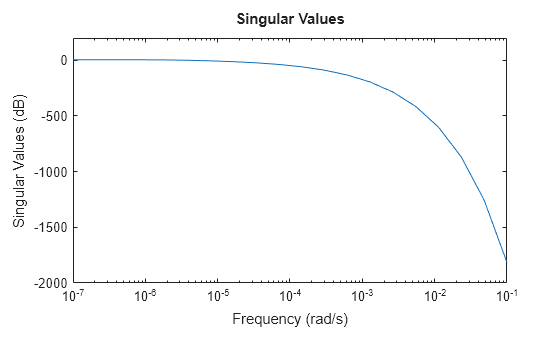
Um eine verkürzte Annäherung zu erhalten, verwenden Sie zpk und geben Sie das Frequenzband des Fokus an. Bei diesem Modell können Sie einen Frequenzbereich von 0 rad/s bis 0.01 rad/s verwenden, um die Näherung niedriger Ordnung zu erhalten.

zsys = zpk(sys,Focus=[0 1e-2],Display="off");

Vergleichen Sie den Frequenzgang.

sigmaplot(sys,zsys,w)

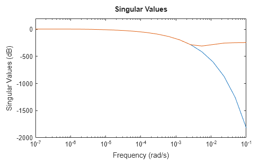
Dieses thermische Modell fällt jenseits von 0.001 rad/s sehr steil ab. Standardmäßig bietet das mit zpk erhaltene reduzierte Modell keine gute Übereinstimmung mit diesem Abfall. Um dies abzumildern, können Sie das Argument RollOff von zpk verwenden und einen minimalen Abfall-Wert jenseits des fokussierten Frequenzbandes angeben. Geben Sie für die Abfallrate einen Wert von -45 an, was einer Rate von mindestens -900 dB/Dekade entspricht.

zsys2 = zpk(sys,Focus=[0 1e-2],RollOff=-45,Display="off");
sigmaplot(sys,zsys2,w)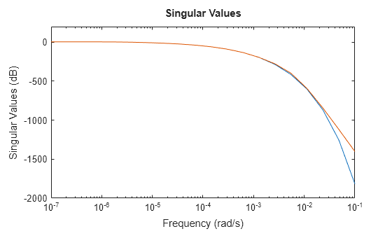

Das reduzierte Modell liefert nun eine viel bessere Annäherung an den Abfall-Wert. In diesem Beispiel führt die Anpassung der Abfallrate mit zpk jedoch dazu, dass die Nullstellen und Polstellen erneut berechnet werden müssen. Dies kann bei großen Modellen sehr rechenintensiv sein. Als Alternative können Sie die Methode der Nullpolabschneidung von reducespec verwenden und den Abfall ohne zusätzliche Berechnungskosten anpassen, nachdem die Software die Polstellen und Nullstellen berechnet hat. Ein Beispiel hierzu finden Sie unter Zero-Pole Truncation of Thermal Model.

Algorithmen

zpk verwendet die MATLAB-Funktion roots, um Transferfunktionen zu konvertieren und die Funktionen zero und pole, um Zustandsraummodelle zu konvertieren.

Zur Konvertierung schwach besetzter Modelle verwendet zpk den Krylov-Schur-Algorithmus [1] für inverse Potenziteration, um Polstellen und Nullstellen im angegebenen Frequenzband zu berechnen.

Referenzen

[1] Stewart, G. W. “A Krylov--Schur Algorithm for Large Eigenproblems.” SIAM Journal on Matrix Analysis and Applications 23, no. 3 (January 2002): 601–14. https://doi.org/10.1137/S0895479800371529.

Erweiterte Fähigkeiten

Automatische Parallelunterstützung

Schnellerer Code durch automatisches, paralleles Rechnen mit der Parallel Computing Toolbox™. (seit R2026a)

Die Funktion zpk weist eine automatische Parallel-Unterstützung zum Berechnen von verkürzten Null-Polstellen-Verstärkungsannäherungen von schwach besetzten Modellen auf. Um Berechnungen parallel durchzuführen, setzen Sie das Argument UseParallel auf "on" oder "auto". Weitere Informationen finden Sie unter Run MATLAB Functions with Automatic Parallel Support (Parallel Computing Toolbox).

Versionsverlauf

Eingeführt vor R2006a

R2026a: Mehr Kontrolle über die parallele Ausführung mit dem Argument UseParallel

Das Name-Wert-Argument UseParallel akzeptiert nun die Werte "off", "auto" oder "on" statt true oder false. Durch diese Änderung können Sie besser steuern, wann ein Parallel-Pool zur parallelen Ausführung verwendet werden soll.

Es wird nicht empfohlen, für das Name-Wert-Argument UseParallel true oder false anzugeben.

Diese Tabelle zeigt, wie Sie je nach Ihrem Ziel Ihren Code aktualisieren.

Ziel	Nicht empfohlen	Empfohlen
Code schreiben, der auf dem MATLAB-Client ausgeführt wird und das integrierte Multithreading verwendet, um die lokalen Ressourcen optimal zu nutzen.	sys = zpk(sparseSys,UseParallel=false)	sys = zpk(sparseSys,UseParallel="off") (Standard)
Portablen Code schreiben, der in einem Parallel-Pool ausgeführt wird und auf dem MATLAB-Client ausgeführt wird, wenn kein Pool verfügbar ist.	sys = zpk(sparseSys,UseParallel=true)	sys = zpk(sparseSys,UseParallel="auto")
Code schreiben, der in einem Parallel-Pool ausgeführt wird und einen Fehler ausgibt, wenn kein Pool verfügbar ist.	–	sys = zpk(sparseSys,UseParallel="on")

Es wird nicht geplant, die Unterstützung für die Werte true und false aufzugeben.

R2025a: Berechnen einer verkürzten Null-Polstellen-Verstärkungs-Annäherung schwach besetzter Modelle

Sie können nun mit zpk schwach besetzte Zustandsraummodelle konvertieren und eine verkürzte Null-Polstellen-Verstärkungs-Annäherung erhalten. zpk berechnet eine Teilmenge der Nullstellen und Polstellen von schwach besetzten Modellen, typischerweise in einem bestimmten niederfrequenten Band [0 f_max]. Dies kann zu einer besseren Annäherung an niedrige Frequenzen führen als die Reduzierung der Modellordnung durch modale Trunkierung – allerdings auf Kosten eines höheren Rechenaufwands. zpk bietet auch eine direkte Kontrolle über die Abfallrate über die Frequenz f_max hinaus. Verwenden Sie die neue Syntax zsys = zpk(sparseSys,Name=Value), um eine Annäherung zu erhalten, die auf bestimmten Optionen basiert, wie z. B. dem Frequenzbereich des Fokus. Ein Beispiel hierzu finden Sie unter Berechnen einer verkürzten ZPK-Annäherung eines schwach besetzten Modells.

Siehe auch

filt | frd | get | set | ss | zpkdata | genss | tf | realp | genmat

Themen

• Transferfunktionen
• What Are Model Objects?
• Discrete-Time Numeric Models
• Using the Right Model Representation
• FEEDBACK zum Schließen von Rückkopplungsschleifen verwenden