kalman
Design Kalman filter for state estimation
Syntax
Description
[
creates a Kalman filter given the plant model kalmf,L,P] = kalman(sys,Q,R,N)sys and the noise
covariance data Q, R, and N.
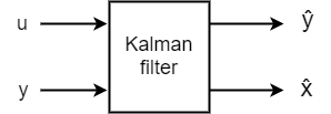
The function computes a Kalman filter for use in a Kalman estimator with the configuration
shown in the following diagram.
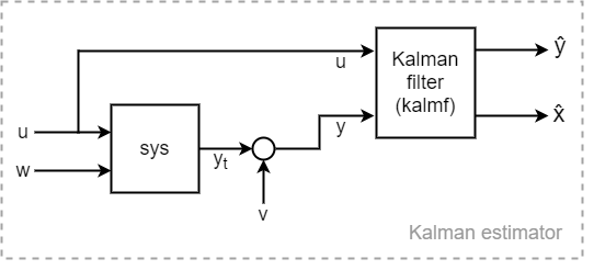
You construct the model sys with known inputs u
and white process noise inputs w, such that w consists
of the last Nw inputs to sys.
The "true" plant output yt consists of all outputs
of sys. You also provide the noise covariance data
Q, R, and N. The returned
Kalman filter kalmf is a state-space model that takes the known inputs
u and the noisy measurements y and produces an
estimate of the true plant output and an estimate of the plant states. kalman also returns the Kalman
gains L and the steady-state error covariance matrix
P.
[
computes a Kalman filter when one or both of the following conditions exist.kalmf,L,P] = kalman(sys,Q,R,N,sensors,known)
Not all outputs of
sysare measured.The disturbance inputs w are not the last inputs of
sys.
The index vector sensors specifies which outputs of
sys are measured. These outputs make up y. The
index vector known specifies which inputs are known (deterministic).
The known inputs make up u. The kalman command takes
the remaining inputs of sys to be the stochastic inputs
w.
[
specifies the estimator type for a discrete-time kalmf,L,P,Mx,Z,My] = kalman(___,type)sys.
type = 'current'— Compute output estimates and state estimates using all available measurements up to .type = 'delayed'— Compute output estimates and state estimates using measurements only up to . The delayed estimator is easier to implement inside control loops.
You can use the type input argument with any of the
previous input argument combinations.
Examples
Design a Kalman filter for a plant that has additive white noise w on the input and v on the output, as shown in the following diagram.
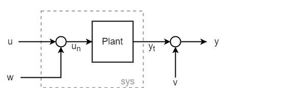
Assume that the plant has the following state-space matrices and is a discrete-time plant with an unspecified sample time (Ts = -1).
A = [1.1269   -0.4940    0.1129
     1.0000         0         0
          0    1.0000         0];

B = [-0.3832
      0.5919
      0.5191];

C = [1 0 0];

D = 0;

Plant = ss(A,B,C,D,-1);
Plant.InputName = 'un';
Plant.OutputName = 'yt';
To use kalman, you must provide a model sys that has an input for the noise w. Thus, sys is not the same as Plant, because Plant takes the input un = u + w. You can construct sys by creating a summing junction for the noise input.
Sum = sumblk('un = u + w');
sys = connect(Plant,Sum,{'u','w'},'yt');
Equivalently, you can use sys = Plant*[1 1].
Specify the noise covariances. Because the plant has one noise input and one output, these values are scalar. In practice, these values are properties of the noise sources in your system, which you determine by measurement or other knowledge of your system. For this example, assume both noise sources have unit covariance and are not correlated (N = 0).
Q = 1;
R = 1;
N = 0;
Design the filter.
[kalmf,L,P] = kalman(sys,Q,R,N);
size(kalmf)
State-space model with 4 outputs, 2 inputs, and 3 states.
The Kalman filter kalmf is a state-space model having two inputs and four outputs. kalmf takes as inputs the plant input signal u and the noisy plant output . The first output is the estimated true plant output . The remaining three outputs are the state estimates . Examine the input and output names of kalmf to see how kalman labels them accordingly.
kalmf.InputName
ans = 2×1 cell
    {'u' }
    {'yt'}
kalmf.OutputName
ans = 4×1 cell
    {'yt_e'}
    {'x1_e'}
    {'x2_e'}
    {'x3_e'}
Examine the Kalman gains L. For a SISO plant with three states, L is a three-element column vector.
L
L = 3×1

    0.3586
    0.3798
    0.0817
For an example that shows how to use kalmf to reduce measurement error due to noise, see Kalman Filtering.
Consider a plant with three inputs, one of which represents process noise w, and two measured outputs. The plant has four states.
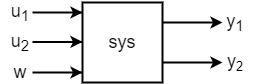
Assuming the following state-space matrices, create sys.
A = [-0.71  0.06 -0.19 -0.17;
      0.06 -0.52 -0.03  0.30;
     -0.19 -0.03 -0.24 -0.02;
     -0.17  0.30 -0.02 -0.41];

B = [ 1.44  2.91   0;
     -1.97  0.83 -0.27;
     -0.20  1.39  1.10;
     -1.2   0    -0.28];

C = [ 0    -0.36 -1.58 0.28;
     -2.05  0     0.51 0.03];

D = zeros(2,3);

sys = ss(A,B,C,D);
sys.InputName = {'u1','u2','w'};
sys.OutputName = {'y1','y2'};
Because the plant has only one process noise input, the covariance Q is a scalar. For this example, assume the process noise has unit covariance.
Q = 1;
kalman uses the dimensions of Q to determine which inputs are known and which are the noise inputs. For scalar Q, kalman assumes one noise input and uses the last input, unless you specify otherwise (see Plant with Unmeasured Outputs).
For the measurement noise on the two outputs, specify a 2-by-2 noise covariance matrix. For this example, use a unit variance for the first output, and variance of 1.3 for the second output. Set the off-diagonal values to zero to indicate that the two noise channels are uncorrelated.
R = [1 0;
     0 1.3];
Design the Kalman filter.
[kalmf,L,P] = kalman(sys,Q,R);
Examine the inputs and outputs. kalman uses the InputName, OutputName, InputGroup, and OutputGroup properties of kalmf to help you keep track of what the inputs and outputs of kalmf represent.
kalmf.InputGroup
ans = struct with fields:
     KnownInput: [1 2]
    Measurement: [3 4]
kalmf.InputName
ans = 4×1 cell
    {'u1'}
    {'u2'}
    {'y1'}
    {'y2'}
kalmf.OutputGroup
ans = struct with fields:
    OutputEstimate: [1 2]
     StateEstimate: [3 4 5 6]
kalmf.OutputName
ans = 6×1 cell
    {'y1_e'}
    {'y2_e'}
    {'x1_e'}
    {'x2_e'}
    {'x3_e'}
    {'x4_e'}
Thus the two known inputs u1 and u2 are the first two inputs of kalmf and the two measured outputs y1 and y2 are the last two inputs to kalmf. For the outputs of kalmf, the first two are the estimated outputs, and the remaining four are the state estimates. To use the Kalman filter, connect these inputs to the plant and noise signals in a manner analogous to that shown for a SISO plant in Kalman Filtering.
Consider a plant with four inputs and two outputs. The first and third inputs are known, while the second and fourth inputs represent the process noise. The plant also has two outputs, but only the second of them is measured.

Use the following state-space matrices to create sys.
A = [-0.37  0.14 -0.01  0.04;
     0.14 -1.89  0.98 -0.11;
    -0.01  0.98 -0.96 -0.14;
     0.04 -0.11 -0.14 -0.95];

B = [-0.07 -2.32  0.68  0.10;
     -2.49  0.08  0     0.83;
      0    -0.95  0     0.54;
     -2.19  0.41  0.45  0.90];

C = [ 0     0    -0.50 -0.38;
     -0.15 -2.12 -1.27  0.65];

D = zeros(2,4);

sys = ss(A,B,C,D,-1);    % Discrete with unspecified sample time

sys.InputName = {'u1','w1','u2','w2'};
sys.OutputName = {'yun','ym'};
To use kalman to design a filter for this system, use the known and sensors input arguments to specify which inputs to the plant are known and which output is measured.
known = [1 3];
sensors = [2];
Specify the noise covariances and design the filter.
Q = eye(2);
R = 1;
N = 0;

[kalmf,L,P] = kalman(sys,Q,R,N,sensors,known);
Examining the input and output labels of kalmf shows the inputs that the filter expects and the outputs it returns.
kalmf.InputGroup
ans = struct with fields:
     KnownInput: [1 2]
    Measurement: 3
kalmf.InputName
ans = 3×1 cell
    {'u1'}
    {'u2'}
    {'ym'}
kalmf takes as inputs the two known inputs of sys and the noisy measured outputs of sys.
kalmf.OutputGroup
ans = struct with fields:
    OutputEstimate: 1
     StateEstimate: [2 3 4 5]
The first output of kalmf is its estimate of the true value of the measured plant output. The remaining outputs are the state estimates.
Input Arguments
Plant model with process noise, specified as a state-space (ss) model. The plant has known inputs u and white process
noise inputs w. The plant output
yt does not include the measurement
noise.
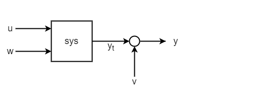
You can write the state-space matrices of such a plant model as:
kalman assumes the Gaussian noise v on the
output. Thus, in continuous time, the state-space equations that
kalman works with are:
In discrete time, the state-space equations are:
If you do not use the known input argument,
kalman uses the size of Q to determine which
inputs of sys are noise inputs. In this case,
kalman treats the last
Nw = size(Q,1) inputs as
the noise inputs. When the noise inputs w are not the last inputs
of sys, you can use the known input argument
to specify which plant inputs are known. kalman treats the
remaining inputs as stochastic.
For additional constraints on the properties of the plant matrices, see Limitations.
Process noise covariance, specified as a scalar or
Nw-by-Nw
matrix, where Nw is the number of noise inputs
to the plant. kalman uses the size of Q to
determine which inputs of sys are noise inputs, taking the last
Nw = size(Q,1) inputs
to be the noise inputs unless you specify otherwise with the known
input argument.
kalman assumes that the process noise w is
Gaussian noise with covariance Q =
E(wwT). When the
plant has only one process noise input, Q is a scalar equal to the
variance of w. When the plant has multiple, uncorrelated noise
inputs, Q is a diagonal matrix. In practice, you determine the
appropriate values for Q by measuring or making educated guesses
about the noise properties of your system.
Measurement noise covariance, specified as a scalar or
Ny-by-Ny
matrix, where Ny is the number of plant
outputs. kalman assumes that the measurement noise
v is white noise with covariance R =
E(vvT). When the
plant has only one output channel, R is a scalar equal to the
variance of v. When the plant has multiple output channels with
uncorrelated measurement noise, R is a diagonal matrix. In
practice, you determine the appropriate values for R by measuring
or making educated guesses about the noise properties of your system.
For additional constraints on the measurement noise covariance, see Limitations.
Noise cross covariance, specified as a scalar or
Nw-by-Ny
matrix. kalman assumes that the process noise w
and the measurement noise v satisfy N =
E(wvT). If the two
noise sources are not correlated, you can omit N, which is
equivalent to setting N = 0. In practice, you determine the
appropriate values for N by measuring or making educated guesses
about the noise properties of your system.
Measured outputs of sys, specified as a vector of indices
identifying which outputs of sys are measured. For instance,
suppose that your system has three outputs, but only two of them are measured,
corresponding to the first and third outputs of sys. In this case,
set sensors = [1 3].
Known inputs of sys, specified as a vector of indices
identifying which inputs are known (deterministic). For instance, suppose that your
system has three inputs, but only the first and second inputs are known. In this case,
set known = [1 2]. kalman interprets any
remaining inputs of sys to be stochastic.
Type of discrete-time estimator to compute, specified as either
'current' or 'delayed'. This input is relevant
only for discrete-time sys.
'current'— Compute output estimates and state estimates using all available measurements up to .'delayed'— Compute output estimates and state estimates using measurements only up to . The delayed estimator is easier to implement inside control loops.
For details about how kalman computes the current and delayed
estimates, see Discrete-Time Estimation.
Output Arguments
Kalman estimator or kalman filter, returned as a state-space (ss)
model. The resulting estimator has inputs and outputs . In other words, kalmf takes as inputs the plant
input u and the noisy plant output y, and produces
as outputs the estimated noise-free plant output and the estimated state values .
kalman automatically sets the InputName,
OutputName, InputGroup, and
OutputGroup properties of kalmf to help you
keep track of which inputs and outputs correspond to which signals.
For the state and output equations of kalmf, see Continuous-Time Estimation and Discrete-Time Estimation.
Filter gains, returned as an array of size Nx-by-Ny, where Nx is the number of states in the plant and Ny is the number of plant outputs. In continuous time, the state equation of the Kalman filter is:
In discrete time, the state equation is:
For details about these expressions and how L is computed, see
Continuous-Time Estimation and Discrete-Time Estimation.
Steady-state error covariances, returned as
Nx-by-Nx,
where Nx is the number of states in the plant.
The Kalman filter computes state estimates that minimize P. In
continuous time, the steady-state error covariance is given by:
In discrete time, the steady-state error covariances are given by:
For further details about these quantities and how kalman uses
them, see Continuous-Time Estimation and Discrete-Time Estimation.
Innovation gains of the state estimators for discrete-time systems, returned as an array.
Mx and My are relevant only when
type = 'current', which is the default
estimator for discrete-time systems. For continuous-time sys or
type = 'delayed', then Mx = My =
[].
For the 'current' type estimator, Mx and
My are the innovation gains in the update equations:
When there is no direct feedthrough from the noise input w to the plant output y (that is, when H = 0, see Discrete-Time Estimation), then , and the output estimate simplifies to .
The dimensions of the arrays Mx and My
depend on the dimensions of sys as follows.
Mx— Nx-by-Ny, where Nx is the number of states in the plant and Ny is the number of outputs.My— Ny-by-Ny.
For details about how kalman obtains Mx
and My, see Discrete-Time Estimation.
Limitations
The plant and noise data must satisfy:
(C,A) is detectable, where:
and , where
has no uncontrollable mode on the imaginary axis in continuous time, or on the unit circle in discrete time.
Algorithms
Version History
Introduced before R2006a