lsim

Compute time response simulation data of dynamic system to arbitrary inputs

Syntax

y = lsim(sys,u,t)

y = lsim(sys,u,t,IC)

y = lsim(sys,u,t,IC,p)

[y,tOut] = lsim(___)

[y,tOut,x] = lsim(___)

[y,tOut,x,pOut] = lsim(sys,u,t,IC,p)

[___] = lsim(___,method)

[y,tOut,x,~,xPODOut] = lsim(___,xPODIn)

[y,tOut,x,~,xPODOut] = lsim(___,xPODIn,method)

lsim(___)

lsim(sys)

Description

Response Data

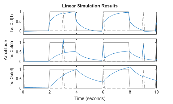
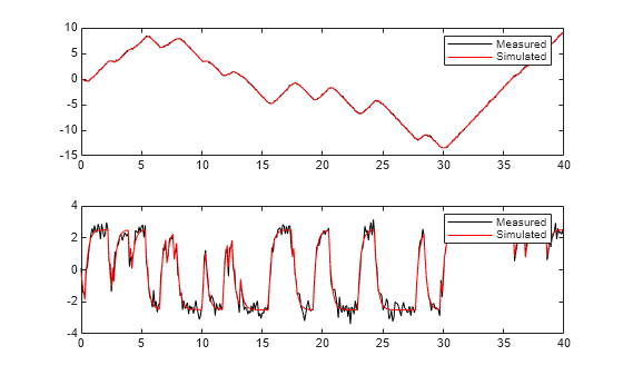
y = lsim(sys,u,t) returns the system response y to the input u, sampled at the same times t as the input. For single-output systems, y is a vector of the same length as t. For multi-output systems, y is an array having as many rows as there are time samples and as many columns as there are outputs in sys.

y = lsim(sys,u,t,IC) further specifies the initial condition IC at t(1), when sys is a state-space model.

y = lsim(sys,u,t,IC,p) specifies the parameter trajectory p when sys is an LPV model. (since R2023a)

[y,tOut] = lsim(___) returns the time samples tOut used for the simulation.

[y,tOut,x] = lsim(___) also returns the state trajectories x, when sys is a state-space model.

[y,tOut,x,pOut] = lsim(sys,u,t,IC,p) returns the parameter trajectories when sys is an LPV model. (since R2023a)

Input Interpolation Method

[___] = lsim(___,method) specifies how lsim interpolates the input values between samples when sys is a continuous-time model.

State Snapshot POD

Since R2024b

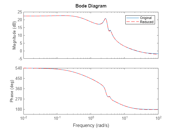
[y,tOut,x,~,xPODOut] = lsim(___,xPODIn) performs proper orthogonal decomposition (POD) of the state snapshots for an LTI state-space model sys. Here, xPOD is an incrementalPOD object. You can start a new POD analysis or add to previous POD results. See incrementalPOD and reducespec for examples and model reduction applications.

[y,tOut,x,~,xPODOut] = lsim(___,xPODIn,method) specifies the input-signal interpolation method when sys is a continuous-time model.

Response Plots

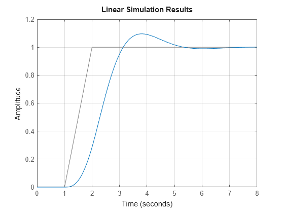
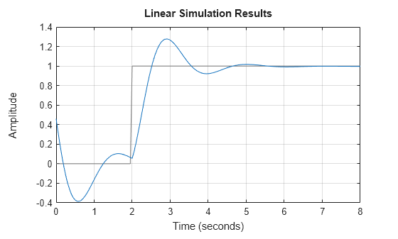
lsim(___) plots the simulated time response of sys to the input history (u,t) for all of the previous input argument combinations except state snapshot POD. The plot uses default plotting options. For more plot customization options, use lsimplot instead.

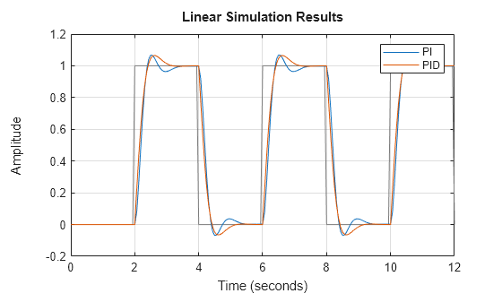
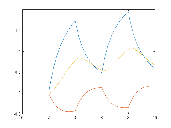
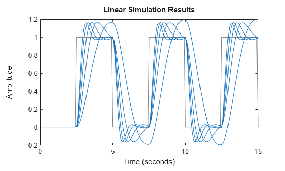
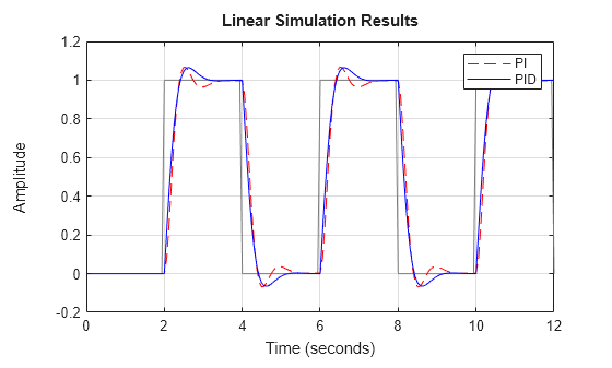
• To plot responses for multiple dynamic systems on the same plot, you can specify sys as a comma-separated list of models. For example, lsim(sys1,sys2,sys3,u,t) plots the responses for three models on the same plot.

• To specify a color, line style, and marker for each system in the plot, specify a LineSpec value for each system. For example, lsim(sys1,LineSpec1,sys2,LineSpec2,u,t) plots two models and specifies their plot style. For more information on specifying a LineSpec value, see lsimplot.

Linear Simulation Tool

lsim(sys) opens the Linear Simulation Tool for simulating sys. For more information about using this tool for linear analysis, see Working with the Linear Simulation Tool.

Examples

Simulated Response to Arbitrary Input Signal

Consider the following transfer function.

sys = tf(3,[1 2 3])

sys =
 
        3
  -------------
  s^2 + 2 s + 3
 
Continuous-time transfer function.

To compute the response of this system to an arbitrary input signal, provide lsim with a vector of the times t at which you want to compute the response and a vector u containing the corresponding signal values. For instance, plot the system response to a ramping step signal that starts at 0 at time t = 0, ramps from 0 at t = 1 to 1 at t = 2, and then holds steady at 1. Define t and compute the values of u.

t = 0:0.04:8;  % 201 points
u = max(0,min(t-1,1));

Use lsim without an output argument to plot the system response to the signal.

lsim(sys,u,t)
grid on

The plot shows the applied input (u,t) in gray and the system response in blue.

Use lsim with an output argument to obtain the simulated response data.

y = lsim(sys,u,t);
size(y)

ans = 1×2

   201     1

The vector y contains the simulated response at the corresponding times in t.

Response to Periodic Signal

Use gensig to create periodic input signals such as sine waves and square waves for use with lsim. Simulate the response to a square wave of the following SISO state-space model.

A = [-3 -1.5; 5 0];
B = [1; 0];
C = [0.5 1.5];
D = 0;
sys = ss(A,B,C,D);

For this example, create a square wave with a period of 10 s and a duration of 20 s.

[u,t] = gensig("square",10,20);

gensig returns the vector t of time steps and the vector u containing the corresponding values of the input signal. (If you do not specify a sample time for t, then gensig generates 64 samples per period.) Use these with lsim and plot the system response.

lsim(sys,u,t)
grid on

The plot shows the applied square wave in gray and the system response in blue. Call lsim with an output argument to obtain the response values at each point in t.

[y,~] = lsim(sys,u,t);

Response of Discrete-Time System

When you simulate the response of a discrete-time system, the time vector t must be of the form Ti:dT:Tf, where dT is the sample time of the model. Simulate the response of the following discrete-time transfer function to a ramp step input.

sys = tf([0.06 0.05],[1 -1.56 0.67],0.05);

This transfer function has a sample time of 0.05 s. Use the same sample time to generate the time vector t and a ramped step signal u.

t = 0:0.05:4;  
u = max(0,min(t-1,1));

Plot the system response.

lsim(sys,u,t)

To simulate the response of a discrete-time system to a periodic input signal, use the same sample time with gensig to generate the input. For instance, simulate the system response to a sine wave with period of 1 s and a duration of 4 s.

[u,t] = gensig("sine",1,4,0.05);

Plot the system response.

lsim(sys,u,t)

Plot Response of Multiple Systems to Same Input

lsim allows you to plot the simulated responses of multiple dynamic systems on the same axis. For instance, compare the closed-loop response of a system with a PI controller and a PID controller. Create a transfer function of the system and tune the controllers.

H = tf(4,[1 10 25]);
C1 = pidtune(H,'PI');
C2 = pidtune(H,'PID');

Form the closed-loop systems.

sys1 = feedback(H*C1,1);
sys2 = feedback(H*C2,1);

Plot the responses of both systems to a square wave with a period of 4 s.

[u,t] = gensig("square",4,12);
lsim(sys1,sys2,u,t)
grid on
legend("PI","PID")

By default, lsim chooses distinct colors for each system that you plot. You can specify colors and line styles using the LineSpec input argument.

 lsim(sys1,"r--",sys2,"b",u,t)
 grid on
 legend("PI","PID")

The first LineSpec "r--" specifies a dashed red line for the response with the PI controller. The second LineSpec "b" specifies a solid blue line for the response with the PID controller. The legend reflects the specified colors and line styles. For more plot customization options, use lsimplot.

Plot Simulated Response of MIMO System

In a MIMO system, at each time step t, the input u(t) is a vector whose length is the number of inputs. To use lsim, you specify u as a matrix with dimensions Nt-by-Nu, where Nu is the number of system inputs and Nt is the length of t. In other words, each column of u is the input signal applied to the corresponding system input. For instance, to simulate a system with four inputs for 201 time steps, provide u as a matrix of four columns and 201 rows, where each row u(i,:) is the vector of input values at the ith time step; each column u(:,j) is the signal applied at the jth input.

Similarly, the output y(t) computed by lsim is a matrix whose columns represent the signal at each system output. When you use lsim to plot the simulated response, lsim provides separate axes for each output, representing the system response in each output channel to the input u(t) applied at all inputs.

Consider the two-input, three-output state-space model with the following state-space matrices.

A = [-1.5  -0.2   1.0;
     -0.2  -1.7   0.6;
      1.0   0.6  -1.4];
  
B = [ 1.5  0.6;
     -1.8  1.0;
      0    0  ];

C = [ 0    -0.5 -0.1;
      0.35 -0.1 -0.15
      0.65  0    0.6];
  
D = [ 0.5  0;
      0.05 0.75
      0    0];

sys = ss(A,B,C,D);

Plot the response of sys to a square wave of period 4 s, applied to the first input sys and a pulse applied to the second input every 3 s. To do so, create column vectors representing the square wave and the pulsed signal using gensig. Then stack the columns into an input matrix. To ensure the two signals have the same number of samples, specify the same end time and sample time.

Tf = 10;
Ts = 0.1;
[uSq,t] = gensig("square",4,Tf,Ts);
[uP,~] = gensig("pulse",3,Tf,Ts);
u = [uSq uP];
lsim(sys,u,t)

Each axis shows the response of one of the three system outputs to the signals u applied at all inputs. Each plot also shows all input signals in gray.

Plot System Evolution from Initial Condition

By default, lsim simulates the model assuming all states are zero at the start of the simulation. When simulating the response of a state-space model, use the optional x0 input argument to specify nonzero initial state values. Consider the following two-state SISO state-space model.

A = [-1.5 -3;
      3   -1];
B = [1.3; 0];
C = [1.15 2.3];
D = 0;
          
sys = ss(A,B,C,D);

Suppose that you want to allow the system to evolve from a known set of initial states with no input for 2 s, and then apply a unit step change. Specify the vector x0 of initial state values, and create the input vector.

x0 = [-0.2 0.3];
t = 0:0.05:8;
u = zeros(length(t),1);
u(t>=2) = 1;
lsim(sys,u,t,x0)
grid on

The first half of the plot shows the free evolution of the system from the initial state values [-0.2 0.3]. At t = 2 there is a step change to the input, and the plot shows the system response to this new signal beginning from the state values at that time.

Extract Simulated Response Data

When you use lsim with output arguments, it returns the simulated response data in an array. For a SISO system, the response data is returned as a column vector of the same length as t. For instance, extract the response of a SISO system to a square wave. Create the square wave using gensig.

sys = tf([2 5 1],[1 2 3]);
[u,t] = gensig("square",4,10,0.05);
[y,t] = lsim(sys,u,t);
size(y)

ans = 1×2

   201     1

The vector y contains the simulated response at each time step in t. (lsim returns the time vector t as a convenience.)

For a MIMO system, the response data is returned in an array of dimensions N-by-Ny-by-Nu, where Ny and Nu are the number of outputs and inputs of the dynamic system. For instance, consider the following state-space model, representing a three-state system with two inputs and three outputs.

A = [-1.5  -0.2   1.0;
     -0.2  -1.7   0.6;
      1.0   0.6  -1.4];
  
B = [ 1.5  0.6;
     -1.8  1.0;
      0    0  ];

C = [ 0   -0.1 -0.2;
      0.7 -0.2 -0.3
     -0.65 0   -0.6];
  
D = [ 0.1  0;
      0.1  1.5
      0    0];

sys = ss(A,B,C,D);

Extract the responses of the three output channels to the square wave applied at both inputs.

uM = [u u];
[y,t] = lsim(sys,uM,t);
size(y)

ans = 1×2

   201     3

y(:,j) is a column vector containing response at the jth output to the square wave applied to both inputs. That is, y(i,:) is a vector of three values, the output values at the ith time step.

Because sys is a state-space model, you can extract the time evolution of the state values in response to the input signal.

[y,t,x] = lsim(sys,uM,t);
size(x)

ans = 1×2

   201     3

Each row of x contains the state values [x1,x2,x3] at the corresponding time in t. In other words, x(i,:) is the state vector at the ith time step. Plot the state values.

plot(t,x)

Response of Systems in Model Array

The example Plot Response of Multiple Systems to Same Input shows how to plot responses of several individual systems on a single axis. When you have multiple dynamic systems arranged in a model array, lsim plots all their responses at once.

Create a model array. For this example, use a one-dimensional array of second-order transfer functions having different natural frequencies. First, preallocate memory for the model array. The following command creates a 1-by-5 row of zero-gain SISO transfer functions. The first two dimensions represent the model outputs and inputs. The remaining dimensions are the array dimensions. (For more information about model arrays and how to create them, see Model Arrays.)

sys = tf(zeros(1,1,1,5));

Populate the array.

w0 = 1.5:1:5.5;    % natural frequencies
zeta = 0.5;        % damping constant
for i = 1:length(w0)
   sys(:,:,1,i) = tf(w0(i)^2,[1 2*zeta*w0(i) w0(i)^2]);
end

Plot the responses of all models in the array to a square wave input.

[u,t] = gensig("square",5,15);
lsim(sys,u,t)

lsim uses the same line style for the responses of all entries in the array. One way to distinguish among entries is to use the SamplingGrid property of dynamic system models to associate each entry in the array with the corresponding w0 value.

sys.SamplingGrid = struct('frequency',w0);

Now, when you plot the responses in a MATLAB® figure window, you can click a trace to see which frequency value it corresponds to.

Simulate Response of Identified Model

Load estimation data to estimate a model.

load dcmotordata
z = iddata(y,u,0.1,'Name','DC-motor');

z is an iddata object that stores the one-input two-output estimation data with a sample time of 0.1 s.

Estimate a state-space model of order 4 using estimation data z.

[sys,x0] = n4sid(z,4);

sys is the estimated model and x0 is the estimated initial states.

Simulate the response of sys using the same input data as the one used for estimation and the initial states returned by the estimation command.

[y,t,x] = lsim(sys,z.InputData,[],x0);

Here, y is the system response, t is the time vector used for simulation, and x is the state trajectory.

Compare the simulated response y to the measured response z.OutputData for both outputs.

subplot(211), plot(t,z.OutputData(:,1),'k',t,y(:,1),'r')
legend('Measured','Simulated')
subplot(212), plot(t,z.OutputData(:,2),'k',t,y(:,2),'r')
legend('Measured','Simulated')

Time Response of Linear-Parameter Varying State-Space Model

For this example, fcnMaglev.m defines the matrices and offsets of a magnetic levitation system. The magnetic levitation controls the height of a levitating ball using a coil current that creates a magnetic force on the ball. This example simulates the model in open loop.

Create an LPV model.

lpvSys = lpvss('h',@fcnMaglev)

Continuous-time state-space LPV model with 1 outputs, 1 inputs, 2 states, and 1 parameters.

You can set additional properties using the dot notation.

lpvSys.StateName = {'h','hdot'};
lpvSys.InputName = 'current';
lpvSys.InputName = 'height';

Simulate the response of this model to an arbitrary sinusoidal input current.

h0 = 1;
[~,~,~,~,~,~,x0,u0,~] = fcnMaglev([],h0);
ic = findop(lpvSys,0,h0,x=x0,u=u0);
t = 0:1e-3:1;
u = u0*(1+0.1*sin(10*t));
y = lsim(lpvSys,u,t,ic,@(t,x,u) x(1));

Plot the response.

plot(t,y,t,u/u0)
legend('height','current')

The ball is attracted to the magnet when the current first increases (h decreases). The subsequent decrease in current is not enough to bring it back.

h = 0 is a singularity for this model, that is, the ball hits the magnet. The LPV model ceases to be valid at this point.

Effect of Sample Time on Simulation

The choice of sample time can drastically affect simulation results. To illustrate why, consider the following second-order model.

$$\begin{array}{cc}sys(s)=\frac{{\omega }^2}{s^2+2s+{\omega }^2},& \omega =62.83\end{array}.$$

Simulate the response of this model to a square wave with period 1 s, using a sample time of 0.1 s.

w2 = 62.83^2;
sys = tf(w2,[1 2 w2]);

tau = 1;
Tf = 5;
Ts = 0.1;
[u,t] = gensig("square",tau,Tf,Ts);
lsim(sys,u,t)

lsim simulates the model using the specified input signal, but it issues a warning that the input signal is undersampled. lsim recommends a sample time that generates at least 64 samples per period of the input u. To see why this recommendation matters, simulate sys again using a sample time smaller than the recommended maximum.

figure
Ts2 = 0.01;
[u2,t2] = gensig("square",tau,Tf,Ts2);
lsim(sys,u2,t2)

This response exhibits strong oscillatory behavior that is hidden in the undersampled version.

Proper Orthogonal Decomposition with Custom Simulations

This example shows how to use custom simulations to obtain state-snapshot data and perform POD model order reduction. By default, the POD algorithm provides three types of built-in excitation signals (chirp, impulse, and PRBS) to perform simulations. The software simulates the model and extracts state-snapshot data and approximates the controllability and observability Gramians. Alternatively, you can provide custom POD data generated from a simulation with incrementalPOD and lsim.

Generate a random state-space model with 30 states, one input, and one output and create a model order reduction task.

rng(0)
sys = rss(30,1,1);
R = reducespec(sys,"pod");

For this example, create a superimposed sinusoidal signal as an input signal for running simulations.

t = linspace(0,100,10000);
u = 0.5*(sin(1.*t)+sin(3.*t)+sin(5.*t)+sin(8.*t)+sin(10.*t));

Create incremental POD objects to store the approximation of reachability and observability Gramians.

rPOD = incrementalPOD;
oPOD = incrementalPOD;

Perform simulations of the plant model and its adjoint with the custom input signal u.

[~,~,~,~,rPOD] = lsim(sys,u,t,rPOD);
asys = adjoint(sys);
[~,~,~,~,oPOD] = lsim(asys,u,t,oPOD);

lsim generates the state-snapshot data and returns the custom POD data as output. This data is generated in a format compatible with R.Options.

Specify the custom data and run the model reduction algorithm. When you specify options CustomLr and CustomLo, the software bypasses the built in simulations and uses the data as is.

R.Options.CustomLr = rPOD;
R.Options.CustomLo = oPOD;
R = process(R);

You can now follow the typical workflow selecting the order and obtaining the reduced order model.

Obtain a reduced-order model that neglects 0.01% of the total energy.

rsys = getrom(R,MaxLoss=1e-4);
order(rsys)

ans = 
9

bodeplot(sys,rsys,"r--")
legend("Original","Reduced")

ans = 
  Legend (Original, Reduced) with properties:

         String: {'Original'  'Reduced'}
       Location: 'northeast'
    Orientation: 'vertical'
       FontSize: 8.1000
       Position: [0.7707 0.8532 0.1875 0.0923]
          Units: 'normalized'

  Show all properties

The reduced model provides a good approximation of the full-order model.

Input Arguments

sys — Dynamic system

dynamic system model | model array

Dynamic system, specified as a SISO or MIMO dynamic system model or array of dynamic system models. Dynamic systems that you can use include:

• Continuous-time or discrete-time numeric LTI models, such as tf, zpk, or ss models.

• Generalized or uncertain LTI models such as genss or uss models. (Using uncertain models requires Robust Control Toolbox™ software.)

  • For tunable control design blocks, the function evaluates the model at its current value for both plotting and returning response data.

  • For uncertain control design blocks, the function plots the nominal value and random samples of the model. When you use output arguments, the function returns response data for the nominal model only.

• Sparse state-space models such as sparss and mechss models.

• Identified LTI models, such as idtf, idss, or idproc models. For such models, the function can also plot confidence intervals and return standard deviations of the frequency response. See Step Responses of Identified Models with Confidence Regions. (Using identified models requires System Identification Toolbox™ software.)

• Linear time-varying (ltvss) and linear parameter-varying (lpvss) models.

This function does not support frequency-response data models such as frd, genfrd, or idfrd models.

If sys is an array of models, the function plots the responses of all models in the array on the same axes. See Step Response of Systems in a Model Array.

u — Input signal

vector | array

Input signal for simulation, specified as one of the following:

• For single-input systems, u is a vector of the same length as t.

• For multi-input systems, u is an array with as many rows as there are time samples (length(t)) and as many columns as there are inputs to sys. In other words, each row u(i,:) represents the values applied at the inputs of sys at time t(i). Each column u(:,j) is the signal applied to the jth input of sys.

t — Time samples

vector

Time samples at which to compute the response, specified as a vector of the form T0:dT:Tf. The lsim command interprets t as having the units specified in the TimeUnit property of the model sys.

For continuous-time sys, the lsim command uses the time step dT to discretize the model. If dT is too large relative to the system dynamics (undersampling), lsim issues a warning recommending a faster sampling time. For further discussion of the impact of sampling time on simulation, see Effect of Sample Time on Simulation.

For discrete-time sys, the time step dT must equal the sample time of sys. Alternatively, you can omit t or set it to []. In that case, lsim sets t to a vector of the same length as u that begins at 0 with a time step equal to sys.Ts.

IC — Initial condition

vector of zeros (default) | vector | operating condition created with findop

Since R2024b

Initial conditions for simulating a state-space model, specified as one of the following:

• A vector xinit having one entry for each state in sys.

• An operating condition obtained with findop. An operating point object allows you to start the simulation from a steady-state operating condition with nonzero past u, w, and y values. For example, to start a simulation from nonzero y value, you can specify:

  op = findop(sys,y=3);
  y = lsim(sys,u,t,op)

If you omit this argument, then the simulation starts from the all-zero initial condition.

p — LPV model parameter trajectory

matrix | function handle

Parameter trajectory of the LPV model, specified as a matrix or a function handle.

• For exogenous or explicit trajectories, specify p as a matrix with dimensions N-by-Np, where N is the number of time samples and Np is the number of parameters.

  Thus, the row vector p(i,:) contains the parameter values at the ith time step.

• For endogenous or implicit trajectories, specify p as a function handle of the form p = F(t,x,u) in continuous time and p = F(k,x,u) in discrete time that gives parameters as a function of time t or time sample k, state x, and input u.

  This option is useful when you want to simulate quasi-LPV models.

method — Discretization method

"zoh" | "foh"

Discretization method for sampling continuous-time models, specified as one of the following.

• "zoh" — Zero-order hold

• "foh" — First-order hold

When sys is a continuous-time model, lsim computes the time response by discretizing the model using a sample time equal to the time step dT = t(2)-t(1) of t. If you do not specify a discretization method, then lsim selects the method automatically based on the smoothness of the signal u. For more information about these two discretization methods, see Continuous-Discrete Conversion Methods.

xPODIn — Proper orthogonal decomposition analysis

incrementalPOD object

Since R2024b

Proper orthogonal decomposition analysis, specified as an incrementalPOD object. Use POD analysis with lsim when you want to bypass the built-in excitation provided by ProperOrthogonalDecomposition model-order specification and provide your own state-snapshot data generated with custom excitations.

You can specify the input xPODIn as a blank incrementalPOD object to start a new analysis or add to an object returned by a previous simulation. Each simulation updates and enriches the POD with more state data.

Output Arguments

y — Simulated response data

array

Simulated response data, returned as an array.

• For single-input systems, y is a column vector of the same length as t.

• For multi-output systems, y is an array with as many rows as there are time samples (length(t)) and as many columns as there are outputs in sys. Thus, the jth column of y, or y(:,j), contains the response at the jth output to u applied at all inputs.

tOut — Time vector

vector

Time vector used for simulation, returned as a column vector. When you specify an input time vector t of the form 0:dT:Tf, then tOut = t. If t is nearly equisampled, lsim adjusts the sample times for simulation and returns the result in tOut. For discrete-time sys, you can omit t or set it to []. In that case, lsim sets t to a vector of the same length as u that begins at 0 with a time step equal to sys.Ts, and returns the result in tOut.

x — State trajectories

array

State trajectories, returned as an array. When sys is a state-space model, x contains the evolution of the states of sys in response to the input. x is an array with as many rows as there are time samples (length(t)) and as many columns as there are states in sys.

pOut — Parameter trajectories

array

Parameter trajectories, returned as an array. When sys is a linear-parameter varying (lpvss) model, pOut contains the evolution of the parameters of sys. pOut is an array with as many rows as there are time samples (length(t)) and as many columns as there are parameters in sys.

xPODOut — Proper orthogonal decomposition analysis

incrementalPOD object

Since R2024b

Proper orthogonal decomposition analysis, returned as an incrementalPOD object.

lsim updates xPODIn with more state data based on the simulation and returns the result in xPODOut. To further update and enrich the POD state, pass xPODOut to subsequent lsim simulations.

Algorithms

For a discrete-time transfer function,

$$sys\left(z^{-1}\right)=\frac{a_0+a_1{z}^{-1}+\dots +a_n{z}^{-n}}{1+b_1{z}^{-1}+\dots +b_n{z}^{-n}},$$

lsim filters the input based on the recursion associated with this transfer function:

$$y\left[k\right]=a_{0}u\left[k\right]+\dots +a_{n}u\left[k-n\right]-b_{1}y\left[k-1\right]-\dots -b_n\left[k-n\right].$$

For discrete-time zpk models, lsim filters the input through a series of first-order or second-order sections. This approach avoids forming the numerator and denominator polynomials, which can cause numerical instability for higher-order models.

For discrete-time state-space models, lsim propagates the discrete-time state-space equations,

$$\begin{array}{c}x\left[n+1\right]=Ax\left[n\right]+Bu\left[n\right],\\ y\left[n\right]=Cx\left[n\right]+Du\left[n\right].\end{array}$$

For continuous-time systems, lsim first discretizes the system using c2d, and then propagates the resulting discrete-time state-space equations. Unless you specify otherwise with the method input argument, lsim uses the first-order-hold discretization method when the input signal is smooth, and zero-order hold when the input signal is discontinuous, such as for pulses or square waves. The sample time for discretization is the spacing dT between the time samples you supply in t.

For continuous-time sparse and LTV and LPV models, lsim uses fixed-step solvers based on the trbdf or hht methods (see SolverOptions property of sparss and mechss models).

Version History

Introduced before R2006a

R2024b: Perform POD analysis of state snapshots using new syntax

Use the new syntax to perform proper orthogonal decomposition (POD) of state snapshots during your custom simulation for a POD model order reduction application (see reducespec and incrementalPOD). To start a new POD analysis or add to previous POD results, use the syntax [y,t,x,~,xPOD] = lsim(sys,__,xPOD), where xPOD is an incrementalPOD object.

R2024b: Specify initial conditions using findop

You can now also specify initial conditions using an operating point object computed using findop. This allows you to start the simulation from a steady-state operating condition with nonzero past u, w, and y values for models with delays. As a result of this change, x0 argument is renamed to IC.