mechss
Sparse second-order state-space model
Description
Use mechss to represent second-order sparse models using
matrices obtained from your finite element analysis (FEA) package. Such sparse models arise
from finite element analysis (FEA) and are useful in fields like structural analysis, fluid
flow, heat transfer, and electromagnetics. The resultant matrices from this type of modeling
are quite large with a sparse pattern. Hence, using mechss is an efficient
way to represent such large sparse state-space models in MATLAB® to perform linear analysis. You can also use mechss to
convert a first-order sparss model object or other dynamic system models to a mechss
object.
You can use mechss model objects to represent SISO or MIMO state-space
models in continuous time or discrete time. In continuous time, a second-order sparse
mass-spring-damper model is represented in the following form:
Here, the full state vector is given by where and are the displacement and velocity vectors. u and
y represent the inputs and outputs, respectively. M,
C and K represent the mass, damping and stiffness
matrices, respectively. B is the input matrix while F
and G are the output matrices for displacement and velocity, respectively.
D is the input-to-output matrix.
You can use a mechss object to:
Perform time-domain and frequency-domain response analysis.
Specify signal-based connections with other LTI models.
Specify physical interfaces between components using the
addInterfaceandassemblecommands.
For more information, see Sparse Model Basics.
Creation
Syntax
Description
sys = mechss(M,C,K,B,F,G,D)mechss object representing this continuous-time
second-order mass-spring-damper model:
Here, M, C, and
K represent the mass, damping, and stiffness matrices,
respectively. B is the input-to-state matrix while
F and G are the displacement-to-output and
velocity-to-output matrices resulting from the two components of the state
x. D is the input-to-output matrix. You can set
M to [] when the mass matrix is an identity
matrix. Set G and D to []
or omit them when they are empty.
sys = mechss(___,PropertyName=Value)
Input Arguments
Mass matrix, specified as an Nq-by-Nq sparse
matrix, where Nq is the number of degrees of freedom. This input
sets the value of property M.
Damping matrix, specified as an Nq-by-Nq
sparse matrix, where Nq is the number of degrees of freedom. You
can also set C=[] to specify zero damping. This input sets the
value of property C.
Stiffness matrix, specified as an Nq-by-Nq
sparse matrix, where Nq is the number of degrees of freedom. This
input sets the value of property K.
Input-to-state matrix, specified as an
Nq-by-Nu sparse matrix, where
Nq is the number of degrees of freedom and Nu
is the number of inputs. This input sets the value of property B.
Displacement-to-output matrix, specified as an
Ny-by-Nq sparse matrix, where
Nq is the number of degrees of freedom and Ny
is the number of outputs. This input sets the value of property F.
Velocity-to-output matrix, specified as an
Ny-by-Nq sparse matrix, where
Nq is the number of degrees of freedom and Ny
is the number of outputs. This input sets the value of property G.
Input-to-output matrix, specified as an
Ny-by-Nu sparse matrix, where
Ny is the number of outputs and Nu is the
number of inputs. This input sets the value of property D.
Sample time, specified as a scalar. For more information see the Ts property.
Output Arguments
Output system model, returned as a mechss model object.
Properties
Mass matrix, specified as an Nq-by-Nq sparse
matrix where, Nq is the number of degrees of freedom.
Damping matrix, specified as an Nq-by-Nq
sparse matrix where, Nq is the number of degrees of freedom.
Damping matrix, specified as an Nq-by-Nq
sparse matrix where, Nq is the number of degrees of freedom.
Input-to-state matrix, specified as an
Nq-by-Nu sparse matrix where,
Nq is the number of degrees of freedom and Nu is
the number of inputs.
Displacement-to-output matrix, specified as an
Ny-by-Nq sparse matrix where,
Nq is the number of degrees of freedom and Ny is
the number of outputs.
Velocity-to-output matrix, specified as an
Ny-by-Nq sparse matrix where,
Nq is the number of degrees of freedom and Ny is
the number of outputs.
Input-to-output matrix, specified as an
Ny-by-Nu sparse matrix where,
Ny is the number of outputs and Nu is the number
of inputs. D is also called the static gain matrix, and represents
the ratio of the output to the input in steady state condition.
State partition information containing state vector components, interfaces between components and internal signal connecting components, specified as a structure array with the following fields:
Type— Type includes component, signal or physical interfaceName— Name of the component, signal or physical interfaceSize— Number of states or degrees of freedom in the partition
You can view the partition information of the sparse state-space model
using showStateInfo. You can also sort and order the partitions in your sparse
model using xsort.
Options for model analysis, specified as a structure with the following fields:
UseParallel— Set this option totrueto enable parallel computing andfalseto disable it. Parallel computing is disabled by default. TheUseParalleloption requires a Parallel Computing Toolbox™ license.DAESolver— Use this option to select the type of differential algebraic equation (DAE) solver. The following DAE solvers are available:'trbdf2'— Fixed-step solver with an accuracy ofo(h^2), wherehis the step size.[2] This is the default solver for themechssmodel object.'trbdf3'— Fixed-step solver with an accuracy ofo(h^3), wherehis the step size.'hht'— Fixed-step solver with an accuracy ofo(h^2), wherehis the step size.[1]
Reducing the step size increases accuracy and extends the frequency range where numerical damping is negligible.
'hht'is the fastest but can run into difficulties with high initial acceleration (for example, an impulse response with initial jerk).'trbdf2'requires about twice as many computations as'hht'and'trbdf3'requires another 50% more computations than'trbdf2'.For an example, see Time and Frequency Response of Sparse Second-Order Model.
Internal delays in the model, specified as a vector. Internal delays arise, for example, when closing feedback loops on systems with delays, or when connecting delayed systems in series or parallel. For more information about internal delays, see Closing Feedback Loops with Time Delays.
For continuous-time models, internal delays are expressed in the time unit specified by the TimeUnit property of the model. For discrete-time models, internal delays are expressed as integer multiples of the sample time Ts. For example, InternalDelay = 3 means a delay of three sampling periods.
You can modify the values of internal delays using the property InternalDelay. However, the number of entries in sys.InternalDelay cannot change, because it is a structural property of the model.
Input delay for each input channel, specified as one of the following:
Scalar — Specify the input delay for a SISO system or the same delay for all inputs of a multi-input system.
Nu-by-1 vector — Specify separate input delays for input of a multi-input system, whereNuis the number of inputs.
For continuous-time systems, specify input delays in the time unit specified by the TimeUnit property. For discrete-time systems, specify input delays in integer multiples of the sample time, Ts.
For more information, see Time Delays in Linear Systems.
Output delay for each output channel, specified as one of the following:
Scalar — Specify the output delay for a SISO system or the same delay for all outputs of a multi-output system.
Ny-by-1 vector — Specify separate output delays for output of a multi-output system, whereNyis the number of outputs.
For continuous-time systems, specify output delays in the time unit specified by the TimeUnit property. For discrete-time systems, specify output delays in integer multiples of the sample time, Ts.
For more information, see Time Delays in Linear Systems.
Sample time, specified as:
0for continuous-time systems.A positive scalar representing the sampling period of a discrete-time system. Specify
Tsin the time unit specified by theTimeUnitproperty.-1for a discrete-time system with an unspecified sample time.
Time variable units, specified as one of the following:
'nanoseconds''microseconds''milliseconds''seconds''minutes''hours''days''weeks''months''years'
Changing TimeUnit has no effect on other properties, but changes the overall system behavior. Use chgTimeUnit to convert between time units without modifying system behavior.
Input channel names, specified as one of the following:
A character vector, for single-input models.
A cell array of character vectors, for multi-input models.
'', no names specified, for any input channels.
Alternatively, you can assign input names for multi-input models using automatic vector
expansion. For example, if sys is a two-input model, enter the
following.
sys.InputName = 'controls';The input names automatically expand to {'controls(1)';'controls(2)'}.
You can use the shorthand notation u to refer to the InputName property. For example, sys.u is equivalent to sys.InputName.
Use InputName to:
Identify channels on model display and plots.
Extract subsystems of MIMO systems.
Specify connection points when interconnecting models.
Input channel units, specified as one of the following:
A character vector, for single-input models.
A cell array of character vectors, for multi-input models.
'', no units specified, for any input channels.
Use InputUnit to specify input signal units. InputUnit has no effect on system behavior.
Input channel groups, specified as a structure. Use InputGroup to assign
the input channels of MIMO systems into groups and refer to each group by name. The
field names of InputGroup are the group names and the field values
are the input channels of each group. For example, enter the following to create input
groups named controls and noise that include input
channels 1 and 2, and 3 and
5, respectively.
sys.InputGroup.controls = [1 2];
sys.InputGroup.noise = [3 5];
You can then extract the subsystem from the controls inputs to all outputs
using the following.
sys(:,'controls')By default, InputGroup is a structure with no fields.
Output channel names, specified as one of the following:
A character vector, for single-output models.
A cell array of character vectors, for multi-output models.
'', no names specified, for any output channels.
Alternatively, you can assign output names for multi-output models using automatic vector
expansion. For example, if sys is a two-output model, enter the
following.
sys.OutputName = 'measurements';The output names automatically expand to {'measurements(1)';'measurements(2)'}.
You can also use the shorthand notation y to refer to the OutputName property. For example, sys.y is equivalent to sys.OutputName.
Use OutputName to:
Identify channels on model display and plots.
Extract subsystems of MIMO systems.
Specify connection points when interconnecting models.
Output channel units, specified as one of the following:
A character vector, for single-output models.
A cell array of character vectors, for multi-output models.
'', no units specified, for any output channels.
Use OutputUnit to specify output signal units. OutputUnit has no effect on system behavior.
Output channel groups, specified as a structure. Use OutputGroup to
assign the output channels of MIMO systems into groups and refer to each group by name.
The field names of OutputGroup are the group names and the field
values are the output channels of each group. For example, create output groups named
temperature and measurement that include
output channels 1, and 3 and 5,
respectively.
sys.OutputGroup.temperature = [1];
sys.OutputGroup.measurement = [3 5];
You can then extract the subsystem from all inputs to the measurement
outputs using the following.
sys('measurement',:)By default, OutputGroup is a structure with no fields.
User-specified text that you want to associate with the system, specified as a character vector or cell array of character vectors. For example, 'System is MIMO'.
User-specified data that you want to associate with the system, specified as any MATLAB data type.
System name, specified as a character vector. For example, 'system_1'.
Sampling grid for model arrays, specified as a structure array.
Use SamplingGrid to track the variable values associated with
each model in a model array.
Set the field names of the structure to the names of the sampling variables. Set the field values to the sampled variable values associated with each model in the array. All sampling variables must be numeric scalars, and all arrays of sampled values must match the dimensions of the model array.
For example, you can create an 11-by-1 array of linear
models, sysarr, by taking snapshots of a linear time-varying system
at times t = 0:10. The following code stores the time samples with
the linear models.
sysarr.SamplingGrid = struct('time',0:10)Similarly, you can create a 6-by-9 model array,
M, by independently sampling two variables, zeta
and w. The following code maps the (zeta,w) values
to M.
[zeta,w] = ndgrid(<6 values of zeta>,<9 values of w>)
M.SamplingGrid = struct('zeta',zeta,'w',w)
By default, SamplingGrid is a structure with no fields.
Object Functions
The following lists show functions you can use with mechss model
objects.
sparss | Sparse first-order state-space model |
getx0 | Map initial conditions from a mechss object to a
sparss object |
full | Convert sparse models to dense storage |
imp2exp | Convert implicit linear relationship to explicit input-output relation |
inv | Invert dynamic system models |
getDelayModel | State-space representation of internal delays |
sparssdata | Access first-order sparse state-space model data |
mechssdata | Access second-order sparse state-space model data |
showStateInfo | State vector map for sparse model |
spy | Visualize sparsity pattern of a sparse model |
step | Step response of dynamic system |
impulse | Impulse response plot of dynamic system; impulse response data |
initial | System response to initial states of state-space model |
lsim | Compute time response simulation data of dynamic system to arbitrary inputs |
bode | Bode frequency response of dynamic system |
nyquist | Nyquist response of dynamic system |
nichols | Nichols response of dynamic system |
sigma | Singular values of frequency response of dynamic system |
passiveplot | Compute or plot passivity index as function of frequency |
dcgain | Low-frequency (DC) gain of LTI system |
evalfr | Evaluate system response at specific frequency |
freqresp | Evaluate system response over a grid of frequencies |
addInterface | Add interface for physical assembly |
assemble | Assemble components by connecting their physical interfaces |
xsort | Sort states based on state partition |
feedback | Feedback connection of multiple models |
parallel | Parallel connection of two models |
append | Group models by appending their inputs and outputs |
connect | Block diagram interconnections of dynamic systems |
lft | Generalized feedback interconnection of two models (Redheffer star product) |
series | Series connection of two models |
Examples
For this example, consider the sparse matrices for the 3-D beam model subjected to an impulsive point load at its tip in the file sparseBeam.mat.
Extract the sparse matrices from sparseBeam.mat.
load('sparseBeam.mat','M','K','B','F','G','D');
Create the mechss model object by specifying [] for matrix C, since there is no damping.
sys = mechss(M,[],K,B,F,G,D)
Sparse continuous-time second-order model with 3 outputs, 1 inputs, and 3408 degrees of freedom.
Model Properties

Use "spy" and "showStateInfo" to inspect model structure.
Type "help mechssOptions" for available solver options for this model.
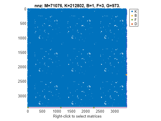
The output sys is a mechss model object containing a 3-by-1 array of sparse models with 3408 degrees of freedom, 1 input, and 3 outputs.
You can use the spy command to visualize the sparsity of the mechss model object.
spy(sys)

For this example, consider the sparse matrices of the discrete system in the file discreteSOSparse.mat.
Load the sparse matrices from discreteSOSparse.mat.
load('discreteSOSparse.mat','M','C','K','B','F','G','D','ts');
Create the discrete-time mechss model object by specifying the sample time ts.
sys = mechss(M,C,K,B,F,G,D,ts)
Sparse discrete-time second-order model with 1 outputs, 1 inputs, and 28408 degrees of freedom.
Model Properties

Use "spy" and "showStateInfo" to inspect model structure.
Type "help mechssOptions" for available solver options for this model.
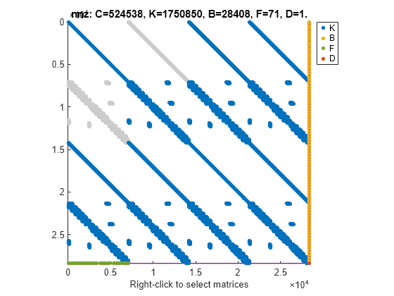
The output sys is a discrete-time mechss model object with 28408 degrees of freedom, 1 input, and 1 output.
You can use the spy command to visualize the sparsity pattern of the mechss model object. You can right-click on the plot to select matrices to be displayed.
spy(sys)

For this example, consider sparseSOArray.mat which contains three sets of sparse matrices that define multiple sparse second-order state-space models.
Extract the data from sparseSOArray.mat.
load('sparseSOArray.mat');Preallocate a 3-by-1 array of mechss models.
sys = mechss(zeros(1,1,3));
Next, use indexed assignment to populate the 3-by-1 array with sparse second-order models.
sys(:,:,1) = mechss(M1,[],K1,B1,F1,G1,[]);
sys(:,:,2) = mechss(M2,[],K2,B2,F2,G2,[]);
sys(:,:,3) = mechss(M3,[],K3,B3,F3,G3,[]);
size(sys)
3x1 array of sparse second-order models.
Each model has 1 outputs, 1 inputs, and between 385 and 738 degrees of freedom.
Alternatively, you can also create an array of sparse second-order models using the stack command when you have models with the same I/O sizes.
Copyright 2020 The MathWorks, Inc
Create a static gain MIMO sparse second-order state-space model.
Consider the following two-input, three-output static gain matrix:
Specify the gain matrix and create the static gain sparse second-order state-space model.
D = [1,5;2,3;5,9];
sys = mechss(D);
size(sys)
Sparse second-order model with 3 outputs, 2 inputs, and 0 degrees of freedom.
For this example, consider sparseSOSignal.mat which contains the mass, stiffness, and damping sparse matrices.
Load the sparse matrices from sparseSOSignal.mat and create the sparse second-order model object.
load('sparseSOModel.mat','M','C','K');
sys = mechss(M,C,K);
mechss creates the model object sys with the following assumptions:
Identity matrices for
BandFwith the same size as mass matrixM.Zero matrices for
GandD.
For this example, consider sparssModel.mat that contains a sparss model object ltiSys.
Load the sparss model object from sparssModel.mat.
load('sparssModel.mat','ltiSys');
ltiSys
Sparse continuous-time state-space model with 1 outputs, 1 inputs, and 354 states.
Model Properties

Use "spy" and "showStateInfo" to inspect model structure.
Type "help sparssOptions" for available solver options for this model.
Use the mechss command to convert to mechss model object representation.
sys = mechss(ltiSys)
Sparse continuous-time second-order model with 1 outputs, 1 inputs, and 354 degrees of freedom.
Model Properties

Use "spy" and "showStateInfo" to inspect model structure.
Type "help mechssOptions" for available solver options for this model.
For this example, consider tuningForkData.mat that contains the sparse second-order model of a tuning fork being struck gently but quickly on one of its tines. The system has one input, the pressure applied on one of its tines, which results in two outputs - the displacements at the tip and base of the tuning fork.
Load the sparse matrices from tuningForkData.mat into the workspace and create the mechss model object.
load('tuningForkData.mat','M','K','B','F');
sys = mechss(M,[],K,B,F,'InputName','pressure','Outputname',{'y tip','x base'})
Next, set solver options for the model by setting the UseParallel parameter to true and the DAESolver to use trbdf3. Use spy to inspect the model structure. Enabling parallel computing requires a Parallel Computing Toolbox™ license.
sys.SolverOptions.UseParallel = true;
sys.SolverOptions.DAESolver = 'trbdf3';
spy(sys)
You can also use showStateInfo to examine the components.
showStateInfo(sys)
Use step to obtain the step response plot of the system. You need to provide the time vector or final time for sparse models.
t = linspace(0,0.5,1000);
step(sys,t)

Next, obtain the Bode plot to examine the frequency response. You need to provide the frequency vector for sparse models.
w = logspace(1,5,1000);
bode(sys,w), grid

For this example, consider sparseSOSignal.mat that contains a sparse second-order model. Define an actuator, sensor, and controller and connect them together with the plant in a feedback loop.
Load the sparse matrices and create the mechss object.
load sparseSOSignal.mat
plant = mechss(M,C,K,B,F,[],[],'Name','Plant');
Next, create an actuator and sensor using transfer functions.
act = tf(1,[1 0.5 3],'Name','Actuator');
sen = tf(1,[0.02 7],'Name','Sensor');
Create a PID controller object for the plant.
con = pid(1,1,0.1,0.01,'Name','Controller');
Use the feedback command to connect the plant, sensor, actuator, and controller in a feedback loop.
sys = feedback(sen*plant*act*con,1)
Sparse continuous-time second-order model with 1 outputs, 1 inputs, and 7111 degrees of freedom.
Model Properties

Use "spy" and "showStateInfo" to inspect model structure.
Type "help mechssOptions" for available solver options for this model.
The resultant system sys is a mechss object since mechss objects take precedence over all other model object types.
Use showStateInfo to view the component and signal groups.
showStateInfo(sys)
The state groups are:

    Type          Name       Size
  -------------------------------
  Component      Sensor         1
  Component      Plant       7102
  Signal                        1
  Component     Actuator        2
  Signal                        1
  Component    Controller       2
  Signal                        1
  Signal                        1
Use xsort to sort the components and signals, and then view the component and signal groups.
sysSort = xsort(sys);
showStateInfo(sysSort)
The state groups are:

    Type          Name       Size
  -------------------------------
  Component      Sensor         1
  Component      Plant       7102
  Component     Actuator        2
  Component    Controller       2
  Signal                        4
Observe that the components are now ordered before the signal partition. The signals are now sorted and grouped together in a single partition.
You can also visualize the sparsity pattern of the resultant system using spy.
spy(sysSort)

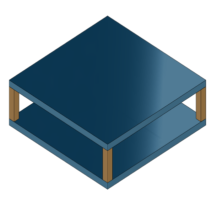
For this example, consider a structural model that consists of two square plates connected with pillars at each vertex as depicted in the figure below. The lower plate is attached rigidly to the ground while the pillars are attached rigidly to each vertex of the square plate.

Load the finite element model matrices contained in platePillarModel.mat and create the sparse second-order model representing the above system.
load('platePillarModel.mat')Define interfaces.
Plate1 = mechss(M1,[],K1,B1,F1,'Name','Plate1');
Plate2 = mechss(M2,[],K2,B2,F2,'Name','Plate2');
Now, load the interfaced degree of freedom (DOF) index data from dofData.mat and use interface to create the physical connections between the two plates and the four pillars. dofs is a 6x7 cell array where the first two rows contain DOF index data for the first and second plates while the remaining four rows contain index data for the four pillars. By default, the function uses dual-assembly method of physical coupling.
load('dofData.mat','dofs')
for ct=1:4
    % Plates to pillars
    Plate1 = addInterface(Plate1,"Pillar"+ct,dofs{1,2+ct});
    Plate2 = addInterface(Plate2,"Pillar"+ct,dofs{2,2+ct});
end

P = cell(4,1);
for ct=1:4
    % Pillars to plates
    P{ct} = mechss(Mp,[],Kp,Bp,Fp,'Name',"Pillar"+ct);
    P{ct} = addInterface(P{ct},"TopMount",dofs{2+ct,1});
    P{ct} = addInterface(P{ct},"BottomMount",dofs{2+ct,2});
end
% Plate 2 to ground
Specify connection between the bottom plate and the ground.
Plate2 = addInterface(Plate2,"Ground",dofs{2,7});

% Assemble
model = append(Plate1,Plate2,P{:});
Use showStateInfo to confirm the physical interfaces.
showStateInfo(model)
The state groups are:

    Type        Name      Size
  ----------------------------
  Component    Plate1     2646
  Component    Plate2     2646
  Component    Pillar1     132
  Component    Pillar2     132
  Component    Pillar3     132
  Component    Pillar4     132
sysConDual = model;
for ct=1:4
    sysConDual = assemble(sysConDual,"Plate1:Pillar"+ct,"Pillar"+ct+":TopMount"');
    sysConDual = assemble(sysConDual,"Plate2:Pillar"+ct,"Pillar"+ct+":BottomMount");
end
sysConDual = assemble(sysConDual,"Plate2:Ground","Ground");
Use showStateInfo to confirm the physical interfaces.
showStateInfo(sysConDual)
The state groups are:

    Type                      Name                   Size
  -------------------------------------------------------
  Component                  Plate1                  2646
  Component                  Plate2                  2646
  Component                 Pillar1                   132
  Component                 Pillar2                   132
  Component                 Pillar3                   132
  Component                 Pillar4                   132
  Interface     Plate1:Pillar1-Pillar1:TopMount        12
  Interface    Plate2:Pillar1-Pillar1:BottomMount      12
  Interface     Plate1:Pillar2-Pillar2:TopMount        12
  Interface    Plate2:Pillar2-Pillar2:BottomMount      12
  Interface     Plate1:Pillar3-Pillar3:TopMount        12
  Interface    Plate2:Pillar3-Pillar3:BottomMount      12
  Interface     Plate1:Pillar4-Pillar4:TopMount        12
  Interface    Plate2:Pillar4-Pillar4:BottomMount      12
  Interface           Plate2:Ground-Ground              6
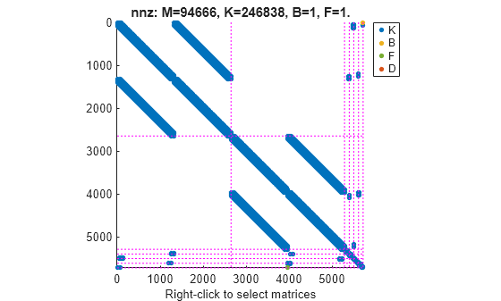
You can use spy to visualize the sparse matrices in the final model.
spy(sysConDual)

Now, specify physical connections using the primal-assembly method.
sysConPrimal = model;
for ct=1:4
    sysConPrimal = assemble(sysConPrimal,"Plate1:Pillar"+ct,"Pillar"+ct+":TopMount"',Method="primal");
    sysConPrimal = assemble(sysConPrimal,"Plate2:Pillar"+ct,"Pillar"+ct+":BottomMount",Method="primal");
end
sysConPrimal = assemble(sysConPrimal,"Plate2:Ground","Ground",Method="primal");
Use showStateInfo to confirm the physical interfaces.
showStateInfo(sysConPrimal)
The state groups are:

    Type       Name    Size
  -------------------------
  Component            5718
Primal assembly eliminates half of the redundant DOFs associated with the shared set of DOFs in the global finite element mesh.
You can use spy to visualize the sparse matrices in the final model.
spy(sysConPrimal)

The data set for this example was provided by Victor Dolk from ASML.
References
[1] H. Hilber, T. Hughes & R. Taylor. " Improved numerical dissipation for time integration algorithms in structural dynamics." Earthquake Engineering and Structural Dynamics, vol. 5, no. 3, pp. 283-292, 1977.
[2] M. Hosea and L. Shampine. "Analysis and implementation of TR-BDF2." Applied Numerical Mathematics, vol. 20, no. 1-2, pp. 21-37, 1996.
Version History
Introduced in R2020b
MATLAB Command
You clicked a link that corresponds to this MATLAB command:
Run the command by entering it in the MATLAB Command Window. Web browsers do not support MATLAB commands.
Website auswählen
Wählen Sie eine Website aus, um übersetzte Inhalte (sofern verfügbar) sowie lokale Veranstaltungen und Angebote anzuzeigen. Auf der Grundlage Ihres Standorts empfehlen wir Ihnen die folgende Auswahl: .
Sie können auch eine Website aus der folgenden Liste auswählen:
So erhalten Sie die bestmögliche Leistung auf der Website
Wählen Sie für die bestmögliche Website-Leistung die Website für China (auf Chinesisch oder Englisch). Andere landesspezifische Websites von MathWorks sind für Besuche von Ihrem Standort aus nicht optimiert.
Amerika
- América Latina (Español)
- Canada (English)
- United States (English)
Europa
- Belgium (English)
- Denmark (English)
- Deutschland (Deutsch)
- España (Español)
- Finland (English)
- France (Français)
- Ireland (English)
- Italia (Italiano)
- Luxembourg (English)
- Netherlands (English)
- Norway (English)
- Österreich (Deutsch)
- Portugal (English)
- Sweden (English)
- Switzerland
- United Kingdom (English)