Main Content

lpvss

Linear parameter-varying state-space model

Since R2023a

    Description

    Use lpvss to represent linear state-space models whose dynamics vary as a function of time-dependent parameters. Linear parameter-varying (LPV) models are helpful to obtain low-complexity, locally linear approximations of nonlinear systems. They can model a much richer class of behaviors than LTI models, especially when the parameters are allowed to depend on internal states (quasi-LPV). Hence, using lpvss models lets you efficiently apply design techniques, such as gain-scheduled control, to nonlinear models.

    You can use lpvss to create continuous-time or discrete-time linear parameter-varying state-space models. In continuous time, an lpvss model is described by the following state-space equations.

    E(t,p)x˙=δ0(t,p)+A(t,p)(xx0(t,p))+B(t,p)(uu0(t,p))y(t)=y0(t,p)+C(t,p)(xx0(t,p))+D(t,p)(uu0(t,p))

    Here, p is a vector of time-dependent exogenous parameters and δ0(t,p), x0(t,p), u0(t,p), and y0(t,p) are varying derivative, state, input, and output offsets, respectively.

    In discrete time, an lpvss model is described by the following state-space equations.

    E(k,pk)xk+1=δ0(k,pk)+A(k,pk)(xkx0(k,pk))+B(k,pk)(uku0(k,pk))yk=y0(k,pk)+C(k,pk)(xkx0(k,pk))+D(k,pk)(uku0(k,pk))

    Here, the integer index k counts the number of sampling periods Ts.

    You can use an lpvss object to model:

    Use lpvss to construct LPV models whose dynamics are described by a MATLAB® function (the data function). Use ssInterpolant to construct LPV models that interpolate linearized LTI dynamics over a grid of operating conditions. The lpvss object cannot represent quasi-LPV models consisting of an LPV model with a scheduling map p(t) = h(t,x,u), but you can specify the parameter trajectory as a function of time t, states x, and inputs u to simulate quasi-LPV models. See LPV and LTV Models for functions and operations applicable to lpvss objects.

    Creation

    Description

    example

    lpvSys = lpvss(ParamNames,DataFcn) creates a continuous-time LPV model. ParamNames specifies a name for each element of the parameter vector p. DataFcn is the name or a handle to the data function, the user-defined MATLAB function that calculates the matrices and offsets for given (t,p) values (or (k,p) values in discrete time).

    example

    lpvSys = lpvss(ParamNames,DataFcn,ts) creates a discrete-time LPV model with sample time ts.

    example

    lpvSys = lpvss(ParamNames,DataFcn,ts,tcheck,pcheck) evaluates DataFcn at (tcheck,pcheck) to determine the number of states, inputs, and outputs. By default, lpvss uses (tcheck,pcheck) = (0,0).

    example

    lpvSys = lpvss(___,Name=Value) sets properties of the linear parameter-varying model using one or more name-value arguments. Use this syntax with any of the previous input-argument combinations.

    Input Arguments

    expand all

    Parameter names, specified as an Np-by-1 cell array of character vectors, where Np is the number of scalar parameters, that is, the number of elements in the parameter vector p. This input sets the value of the property ParameterName.

    User-defined MATLAB function for calculating matrices and offsets, specified as a function name (character vector or string) or a function handle. The data function must be of the following form.

    • Continuous time — [A,B,C,D,E,δ0,x0,u0,y0,Delays]=f(t,p)

    • Discrete time — [A,B,C,D,E,δ0,x0,u0,y0,Delays]=f(k,p)

    The Delay argument is a structure with fields Input and Output specifying the delays in input and output channels, respectively. (since R2024a)

    For more information about defining a data function, see Data Function.

    This input sets the value of property DataFunction.

    Sample time, specified as a scalar. For more information, see the Ts property.

    Test value for time, specified as a scalar. The object evaluates DataFcn at (tcheck,pcheck) to determine the number of states, inputs, and outputs. By default, lpvss uses (tcheck,pcheck) = (0,0).

    Test value for parameters, specified as a scalar or vector of length Np. The object evaluates DataFcn at (tcheck,pcheck) to determine the number of states, inputs, and outputs. By default, lpvss uses (tcheck,pcheck) = (0,0).

    Properties

    expand all

    Names of the parameters in the LPV model, specified as a cell array of character vectors. Specify a cell array of length equal to the length of parameter vector p.

    Data function for calculating the model data, specified as a function handle. The data function must be of the following form.

    • Continuous time

      [A,B,C,D,E,dx0,x0,u0,y0,Delay] = DataFcn(t,p)
    • Discrete time

      [A,B,C,D,E,dx0,x0,u0,y0,Delay] = DataFcn(k,p)

      Here, the input k is an integer index that counts the number of sampling periods Ts. The absolute time is given by t = k*Ts.

    To pass additional input arguments, use an anonymous function as follows.

    DataFcn = @(t) myFunction(t,arg1,arg2,...)

    You can set all output arguments except A, B, C, D to [] when absent for (t,p) values.

    State names, specified as one of the following:

    • Character vector — For first-order models, for example, 'velocity'.

    • Cell array of character vectors — For models with two or more states.

    StateName is empty ' ' for all states by default.

    State path to facilitate state block path management in linearization, specified as one of the following:

    • Character vector — For first-order models

    • Cell array of character vectors — For models with two or more states

    StatePath is empty ' ' for all states by default.

    State units, specified as one of the following:

    • Character vector — For first-order models, for example, 'm/s'

    • Cell array of character vectors — For models with two or more states

    Use StateUnit to keep track of the units of each state. StateUnit has no effect on system behavior. StateUnit is empty ' ' for all states by default.

    Sample time, specified as:

    • 0 for continuous-time systems.

    • A positive scalar representing the sampling period of a discrete-time system. Specify Ts in the time unit specified by the TimeUnit property.

    • -1 for a discrete-time system with an unspecified sample time.

    Note

    Changing Ts does not discretize or resample the model. To convert between continuous-time and discrete-time representations, use c2d and d2c. To change the sample time of a discrete-time system, use d2d.

    Time variable units, specified as one of the following:

    • 'nanoseconds'

    • 'microseconds'

    • 'milliseconds'

    • 'seconds'

    • 'minutes'

    • 'hours'

    • 'days'

    • 'weeks'

    • 'months'

    • 'years'

    Changing TimeUnit has no effect on other properties, but changes the overall system behavior. Use chgTimeUnit to convert between time units without modifying system behavior.

    Input channel names, specified as one of the following:

    • A character vector, for single-input models.

    • A cell array of character vectors, for multi-input models.

    • '', no names specified, for any input channels.

    Alternatively, you can assign input names for multi-input models using automatic vector expansion. For example, if sys is a two-input model, enter the following:

    sys.InputName = 'controls';

    The input names automatically expand to {'controls(1)';'controls(2)'}.

    You can use the shorthand notation u to refer to the InputName property. For example, sys.u is equivalent to sys.InputName.

    Use InputName to:

    • Identify channels on model display and plots.

    • Extract subsystems of MIMO systems.

    • Specify connection points when interconnecting models.

    Input channel units, specified as one of the following:

    • A character vector, for single-input models.

    • A cell array of character vectors, for multi-input models.

    • '', no units specified, for any input channels.

    Use InputUnit to specify input signal units. InputUnit has no effect on system behavior.

    Input channel groups, specified as a structure. Use InputGroup to assign the input channels of MIMO systems into groups and refer to each group by name. The field names of InputGroup are the group names and the field values are the input channels of each group. For example, enter the following to create input groups named controls and noise that include input channels 1 and 2, and 3 and 5, respectively.

    sys.InputGroup.controls = [1 2];
    sys.InputGroup.noise = [3 5];

    You can then extract the subsystem from the controls inputs to all outputs using the following.

    sys(:,'controls')

    By default, InputGroup is a structure with no fields.

    Output channel names, specified as one of the following:

    • A character vector, for single-output models.

    • A cell array of character vectors, for multi-output models.

    • '', no names specified, for any output channels.

    Alternatively, you can assign output names for multi-output models using automatic vector expansion. For example, if sys is a two-output model, enter the following.

    sys.OutputName = 'measurements';

    The output names automatically expand to {'measurements(1)';'measurements(2)'}.

    You can also use the shorthand notation y to refer to the OutputName property. For example, sys.y is equivalent to sys.OutputName.

    Use OutputName to:

    • Identify channels on model display and plots.

    • Extract subsystems of MIMO systems.

    • Specify connection points when interconnecting models.

    Output channel units, specified as one of the following:

    • A character vector, for single-output models.

    • A cell array of character vectors, for multi-output models.

    • '', no units specified, for any output channels.

    Use OutputUnit to specify output signal units. OutputUnit has no effect on system behavior.

    Output channel groups, specified as a structure. Use OutputGroupto assign the output channels of MIMO systems into groups and refer to each group by name. The field names of OutputGroup are the group names and the field values are the output channels of each group. For example, create output groups named temperature and measurement that include output channels 1, and 3 and 5, respectively.

    sys.OutputGroup.temperature = [1];
    sys.OutputGroup.measurement = [3 5];

    You can then extract the subsystem from all inputs to the measurement outputs using the following.

    sys('measurement',:)

    By default, OutputGroup is a structure with no fields.

    System name, specified as a character vector. For example, 'system_1'.

    User-specified text that you want to associate with the system, specified as a character vector or cell array of character vectors. For example, 'System is MIMO'.

    User-specified data that you want to associate with the system, specified as any MATLAB data type.

    Object Functions

    expand all

    sample(Not recommended) Sample linear parameter-varying or time-varying dynamics
    ssInterpolantBuild gridded LTV or LPV model from state-space data
    stepStep response of dynamic system
    impulseImpulse response plot of dynamic system; impulse response data
    lsimPlot simulated time response of dynamic system to arbitrary inputs; simulated response data
    initialSystem response to initial states of state-space model
    feedbackFeedback connection of multiple models
    connectBlock diagram interconnections of dynamic systems
    seriesSeries connection of two models
    parallelParallel connection of two models
    lftGeneralized feedback interconnection of two models (Redheffer star product)
    c2dConvert model from continuous to discrete time
    d2cConvert model from discrete to continuous time
    d2dResample discrete-time model
    xperm Reorder states in state-space models
    sminrealEliminates structurally disconnected states, delays, and blocks

    Examples

    collapse all

    Create a continuous-time SISO linear-parameter varying model.

    For this example, dataFcnMaglev.m defines the matrices and offsets of a magnetic levitation system. The magnetic levitation controls the height of a levitating ball using a coil current that creates a magnetic force on the ball.

    These matrices and offsets are defined in the dataFcnMaglev.m data function provided with this example.

    Create an LPV model.

    lpvsys = lpvss('p',@dataFcnMaglev)
    Continuous-time state-space LPV model with 1 outputs, 1 inputs, 2 states, and 1 parameters.
    Model Properties
    

    View the data function.

    type dataFcnMaglev.m
    function [A,B,C,D,E,dx0,x0,u0,y0,Delays] = dataFcnMaglev(~,p)
    % MAGLEV example:
    % x = [h ; dh/dt]
    % p=hbar (equilibrium height)
    mb = 0.02; % kg
    g = 9.81;
    alpha = 2.4832e-5;
    A = [0 1;2*g/p 0];
    B = [0 ; -2*sqrt(g*alpha/mb)/p];
    C = [1 0];  % h
    D = 0;
    E = [];
    dx0 = [];
    x0 = [p;0];
    u0 = sqrt(mb*g/alpha)*p;  % ibar
    y0 = p;                   % y = h = hbar + (h-hbar)
    Delays = [];
    

    Create a discrete-time linear-parameter varying model.

    The matrices and offsets are given by:

    A=sin(0.1p), B=1, C=1, D=0

    y0=0.1sin(k).

    These matrices and offsets are defined in the lpvFcnDiscrete.m data function provided with this example.

    Specify the properties and create the LPV model.

    Ts = 0.01;
    ParamNames = 'p';
    DataFcn = @lpvFcnDiscrete;
    lpvSys = lpvss(ParamNames,DataFcn,Ts)
    Discrete-time state-space LPV model with 1 outputs, 1 inputs, 1 states, and 1 parameters.
    

    View the data function.

    type lpvFcnDiscrete.m
    function [A,B,C,D,E,dx0,x0,u0,y0,Delays] = lpvFcnDiscrete(k,p)
    A = sin(0.1*p);
    B = 1;
    C = 1;
    D = 0;
    E = [];
    dx0 = [];
    x0 = [];
    u0 = [];
    y0 = 0.1*sin(k);
    Delays = [];
    

    For this example, dataFcnMaglev.m defines the matrices and offsets of a magnetic levitation system. The magnetic levitation controls the height of a levitating ball using a coil current that creates a magnetic force on the ball. This example simulates the model in open loop.

    Create an LPV model.

    lpvSys = lpvss('h',@dataFcnMaglev)
    Continuous-time state-space LPV model with 1 outputs, 1 inputs, 2 states, and 1 parameters.
    Model Properties
    

    You can set additional properties using the dot notation.

    lpvSys.StateName = {'h','hdot'};
    lpvSys.InputName = 'current';
    lpvSys.InputName = 'height';

    Simulate the response of this model to an arbitrary sinusoidal input current.

    h0 = 1;
    [~,~,~,~,~,~,x0,u0,~] = dataFcnMaglev([],h0);
    t = 0:1e-3:1;
    u = u0*(1+0.1*sin(10*t));
    y = lsim(lpvSys,u,t,x0,@(t,x,u) x(1));

    Plot the response.

    plot(t,y,t,u/u0)
    legend('height','current')

    Figure contains an axes object. The axes object contains 2 objects of type line. These objects represent height, current.

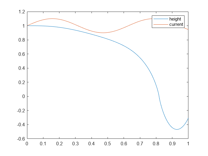
    The ball is attracted to the magnet when the current first increases (h decreases). The subsequent decrease in current is not enough to bring it back.

    h = 0 is a singularity for this model, that is, the ball hits the magnet. The LPV model ceases to be valid at this point.

    You can sample the dynamics of an LPV model over a point or a grid of (t,p) values to obtain affine dynamics for a given time or parameter value.

    For this example, dataFcnMaglev.m defines the matrices and offsets of a magnetic levitation system. The magnetic levitation controls the height of a levitating ball using a coil current that creates a magnetic force on the ball.

    Create an LPV model.

    lpvSys = lpvss('h',@dataFcnMaglev)
    Continuous-time state-space LPV model with 1 outputs, 1 inputs, 2 states, and 1 parameters.
    

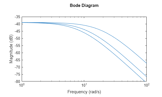
    Sample the LPV dynamics at three h values to obtain local LTI models.

    hmin = 0.05;
    hmax = 0.25;
    hcd = linspace(hmin,hmax,3);
    ssArray = psample(lpvSys,[],hcd);
    size(ssArray)
    1x3 array of state-space models.
    Each model has 1 outputs, 1 inputs, and 2 states.
    

    The function stores the model offsets in the Offsets property of the array.

    ssArray.Offsets
    ans=1×3 struct array with fields:
        dx
        x
        u
        y


    Plot the Bode response.

    bodemag(ssArray)

    View the data function.

    type dataFcnMaglev.m
    function [A,B,C,D,E,dx0,x0,u0,y0,Delays] = dataFcnMaglev(~,p)
    % MAGLEV example:
    % x = [h ; dh/dt]
    % p=hbar (equilibrium height)
    mb = 0.02; % kg
    g = 9.81;
    alpha = 2.4832e-5;
    A = [0 1;2*g/p 0];
    B = [0 ; -2*sqrt(g*alpha/mb)/p];
    C = [1 0];  % h
    D = 0;
    E = [];
    dx0 = [];
    x0 = [p;0];
    u0 = sqrt(mb*g/alpha)*p;  % ibar
    y0 = p;                   % y = h = hbar + (h-hbar)
    Delays = [];
    

    Since R2024a

    This example shows how to create a linear parameter-varying model containing a varying delay. In this example, you also simulate a closed-loop plant with a controller containing an output delay and observe the effects of delayed controller response.

    For this example, dataFcnMaglev.m defines the matrices and offsets of a magnetic levitation system. The magnetic levitation controls the height of a levitating ball using a coil current that creates a magnetic force on the ball.

    Create an LPV model.

    h0 = 1;  % Note: Singular for h=0
    G = lpvss("h",@dataFcnMaglev,0,0,h0);

    This example also provides a data function maglevPD.m which defines a gain-scheduled PD controller for the magnetic levitation plant, containing a time-dependent output delay. This delay decreases with time.

    PD = lpvss("h",@maglevPD,0,0,h0);

    Create the closed-loop response.

    CL = feedback(G*PD,1);

    Simulate the response to the true trajectory p(t)=h(t), which is the first state.

    xinit = [h0;0;0];  % init: h=1
    t = 0:1e-2:10;
    href = h0+0.5*sin(t);  % desired height
    pFcn = @(t,x,u) x(1);
    [y1,~,x1,p1] = lsim(CL,href,t,xinit,pFcn);

    Plot the simulation results and compare to reference height.

    plot(t,href,t,y1,'r--')
    legend("Height reference","LPV simulation")

    Figure contains an axes object. The axes object contains 2 objects of type line. These objects represent Height reference, LPV simulation.

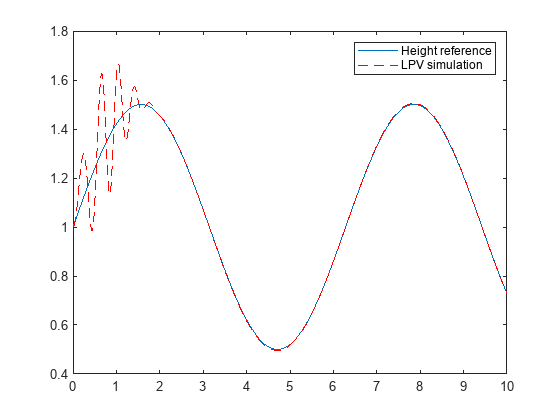
    Because of the delay in controller action, the output signal also has a delayed response of tracking the reference input accurately. As the delay reduces over time, the LPV simulation matches the reference.

    Data Functions

    type dataFcnMaglev.m
    function [A,B,C,D,E,dx0,x0,u0,y0,Delays] = dataFcnMaglev(~,p)
    % MAGLEV example:
    % x = [h ; dh/dt]
    % p=hbar (equilibrium height)
    mb = 0.02; % kg
    g = 9.81;
    alpha = 2.4832e-5;
    A = [0 1;2*g/p 0];
    B = [0 ; -2*sqrt(g*alpha/mb)/p];
    C = [1 0];  % h
    D = 0;
    E = [];
    dx0 = [];
    x0 = [p;0];
    u0 = sqrt(mb*g/alpha)*p;  % ibar
    y0 = p;                   % y = h = hbar + (h-hbar)
    Delays = [];
    
    type maglevPD.m
    function [A,B,C,D,E,dx0,x0,u0,y0,Delays] = maglevPD(t,p)
    % Gain-scheduled PD for MAGLEV example:
    %    dz = A(p) z + B(p) e
    %     u = u0 + C(p) z + D(p) e
    % p=h (equilibrium height)
    mb = 0.02; % kg
    g = 9.81;
    alpha = 2.4832e-5;
    a0 = 2*g/p;
    b0 = -2*sqrt(g*alpha/mb)/p;
    wn = 10;
    zeta = 0.7;
    Kp = (a0+wn^2)/b0;
    Kd = 2*zeta*wn/b0;  % linear in p
    % Kp = (2*zeta*wn-a0)/b0;
    % Kd = wn^2/b0;
    wf = 100;
    A = -wf;
    B = wf;
    C = -wf*Kd;
    D = Kp+wf*Kd;
    E = [];
    dx0 = [];
    x0 = [];
    u0 = [];
    y0 = sqrt(mb*g/alpha)*p;     % ibar, feedforward term
    Delays.Output = 0.1/(1+t);  % decreasing delay
    Delays.Input = NaN;
    end
    

    Version History

    Introduced in R2023a

    expand all