Design and Validate Gain-Scheduled Controller for Nonlinear Aircraft Pitch Dynamics

This example shows how to design and validate gain-scheduled controller for a nonlinear system using a linear parameter-varying state-space model. This example is based on the Approximate Nonlinear Behavior Using Array of LTI Systems (Simulink Control Design) example, and shows how to approximate the nonlinear behavior at the command line.

In this example, you:

1. Linearize a nonlinear Simulink® model on a grid of trim points.

2. Construct an LPV model from the gridded array of LTI models and trim offsets.

3. Design a controller on a grid of trim points. This grid may be different from the grid used for the linearization.

4. Test the controller using command-line LTI simulations (at frozen operating points) and LPV simulations (along a specified parameter trajectory).

5. Test the controller on the nonlinear plant in Simulink.

Aircraft Model

Consider a three-degree-of-freedom model of the pitch axis dynamics of an airframe. The states are the Earth coordinates (${\mathit{X}}_{\mathit{e}}$,${\mathit{Z}}_{\mathit{e}}$), the body coordinates ($\mathit{u}$,$\mathit{w}$), the pitch angle $\theta$, and the pitch rate $\mathit{q}=\dot{\theta }$. This figure summarizes the relationship between the inertial and body frames, the flight path angle $\gamma$, the incidence angle $\alpha$, and the pitch angle $\theta$.

The airframe dynamics are nonlinear and the aerodynamic forces and moments depend on speed $\mathit{V}$ and incidence $\alpha$. The scdairframeOpenLoop model describes these dynamics.

open_system("scdairframeOpenLoop")

Range Of Operating Conditions

Assume that the incidence $\alpha$ varies between –20 and 20 degrees and that the speed $\mathit{V}$ varies between 700 and 1400 m/s. Use a 15-by-12 grid of linearly spaced ($\alpha$,$\mathit{V}$) pairs for scheduling.

nA = 15;   % number of alpha values
nV = 12;   % number of V values
alphaRange = linspace(-20,20,nA)*pi/180;
VRange = linspace(700,1400,nV);
[alpha,V] = ndgrid(alphaRange,VRange);

Batch Trimming

For each flight condition ($\alpha$,$\mathit{V}$), linearize the airframe dynamics at trim (zero normal acceleration and pitching moment). Doing so requires computing the elevator deflection $\delta$ and pitch rate $\mathit{q}$ that result in steady $\mathit{w}$ and $\mathit{q}$.

for ct = 1:nA*nV
   alpha_ini = alpha(ct);      % Incidence [rad]
   v_ini = V(ct);              % Speed [m/s]

   % Specify trim condition
   opspec(ct) = operspec("scdairframeOpenLoop");

   % Xe,Ze: known, not steady.
   opspec(ct).States(1).Known = [1;1];
   opspec(ct).States(1).SteadyState = [0;0];

   % u,w: known, w steady
   opspec(ct).States(3).Known = [1 1];
   opspec(ct).States(3).SteadyState = [0 1];

   % theta: known, not steady
   opspec(ct).States(2).Known = 1;
   opspec(ct).States(2).SteadyState = 0;

   % q: unknown, steady
   opspec(ct).States(4).Known = 0;
   opspec(ct).States(4).SteadyState = 1;

end
opspec = reshape(opspec,[nA nV]);

Trim the model for all of the operating point specifications.

opt = findopOptions("DisplayReport","off","OptimizerType","lsqnonlin");
opt.OptimizationOptions.Algorithm = "trust-region-reflective";
[op,report] = findop("scdairframeOpenLoop",opspec,opt);

Batch Linearization

To linearize the model, first specify linearization input and output points.

io = [linio("scdairframeOpenLoop/delta",1,"in");            % delta
      linio("scdairframeOpenLoop/Airframe Model",1,"out");  % alpha
      linio("scdairframeOpenLoop/Airframe Model",2,"out");  % V
      linio("scdairframeOpenLoop/Airframe Model",3,"out");  % q
      linio("scdairframeOpenLoop/Airframe Model",4,"out");  % az
      linio("scdairframeOpenLoop/Airframe Model",5,"out")]; % gamma

Linearize the model for each of the trim conditions. Store linearization offset information in the info structure.

linOpt = linearizeOptions("StoreOffsets",true);
[G,~,info] = linearize("scdairframeOpenLoop",op,io,linOpt);
G = reshape(G,[nA nV]);
G.u = 'delta';
G.y = {'alpha','V','q','az','gamma'};
G.SamplingGrid = struct("alpha",alpha,"V",V);

G is a 15-by-12 array of linearized plant models at the 180 flight conditions ($\alpha$,$\mathit{V}$).

bodemag(G(3:5,:,:,:))
title("Variations in airframe dynamics")

Use ssInterpolant to construct an LPV model that interpolates these linearized models between grid points.

offsets = info.Offsets;
Glpv = ssInterpolant(G,offsets);

Control Design: Pitch-Axis Stability Augmentation

The ($\alpha$,$\mathit{V}$) grid for control design is coarser and on a smaller range than for the plant model.

nAcd = 5;   % number of alpha values
nVcd = 3;   % number of V values
alphacd = linspace(-10,10,nAcd)*pi/180;
Vcd = linspace(900,1200,nVcd);
[alphacd,Vcd] = ndgrid(alphacd,Vcd);
Ncd = nAcd*nVcd;

Use a 2-DOF gain-scheduled architecture for the pitch rate loop. This combines an I-only term on the error signal $\mathit{e}={\mathit{q}}_{\mathrm{ref}}-\mathit{q}$ with a proportional term on $\mathit{q}$.

$$\delta =\frac{{\mathit{K}}_{\mathit{i}}}{\mathit{s}}\left({\mathit{q}}_{\mathrm{ref}}-\mathit{q}\right)+{\mathit{K}}_{\mathit{p}}\mathit{q}$$

The tunable gains ${\mathit{K}}_{\mathit{p}}$ and ${\mathit{K}}_{\mathit{i}}$ are defined as gain surfaces with a linear dependence on ($\alpha$,$\mathit{V}$).

s = tf("s");
Domain = struct("alpha",alphacd,"V",Vcd);
ShapeFcn = @(x,y) [x y];
Ki = tunableSurface("Ki",-1,Domain,ShapeFcn);
Kp = tunableSurface("Kp",1,Domain,ShapeFcn);
K = [Ki/s Kp] * [1 -1;0 1];
K.InputName = {'qref';'q'};
K.OutputName = {'delta'};

Sample the LPV model of the airframe over the tuning grid (alphacd,Vcd) and build the closed-loop model.

[Ga,Goffsets] = sample(Glpv,[],alphacd,Vcd);
T0 = connect(Ga,K,'qref','q','delta');

Warning: The following block outputs are not used: alpha,V,az,gamma.

Tune the gain surfaces subject to step response and loop-shaping requirements.

R1 = TuningGoal.StepTracking("qref","q",1/2);
R2 = TuningGoal.MaxLoopGain("delta",50,1);
R3 = TuningGoal.MaxGain("qref","q",tf(15,[1 0.01]));
T = systune(T0,[R1 R2],R3);

Final: Soft = 4.94, Hard = 0.19413, Iterations = 30

Warning: StepTracking goal: Feedback configuration has fixed integrators that cannot be stabilized with available tuning parameters. Make sure these are modeling artifacts rather than physical instabilities.

showTunable(T)

Ki =
   -4.4209   -0.0712    1.2825
-----------------------------------
Kp =
    1.1167   -0.0000   -0.2609

View the tuning results.

viewGoal([R1 R2 R3],T)

The tuned gain surfaces show a weak dependence on $\alpha$ and a stronger dependence on $\mathit{V}$.

Ki = setBlockValue(Ki,T);
clf
subplot(211)
viewSurf(Ki)
Kp = setBlockValue(Kp,T);
subplot(212)
viewSurf(Kp)

Build the LPV controller. Include the trim deflection as output offset so that the controller performs an incremental correction around trim.

Ka = ss(setBlockValue(K,T));
Koffsets = reshape(struct("y",{Goffsets.u}),size(Goffsets));
Klpv = ssInterpolant(Ka,Koffsets);

Build the closed-loop LPV model. Note that the plant and controller are sampled and interpolated on two different ($\alpha$,$\mathit{V}$) grids.

Tlpv = feedback(Glpv*Klpv,1,2,3,+1);
Tlpv = Tlpv(:,1); % from qref to plant outputs

Plot the closed-loop responses from ${\mathit{q}}_{\mathrm{ref}}$ to $\mathit{q}$ over the design grid.

clf
step(sample(Tlpv(3,:),[],alphacd,Vcd),6);
grid
title("Closed-loop response qref to q on design grid")

Nonlinear Simulation

To compare the nonlinear and LPV simulation, simulate the step response of the pitch rate loop initialized from one of the trim operating points. This trim condition is chosen on the denser grid and does not belong to the design grid.

aidx = 9;
Vidx = 6;
alpha0 = alphaRange(aidx);
V0 = VRange(Vidx);
q0 = offsets(aidx,Vidx).x(4);

Pick the initial state ${\mathit{x}}_{\mathrm{K0}}$ of the LPV controller to deliver the trim deflection ${\delta }_0$ for the selected operating point. Since the LPV controller output is

$$\delta ={\delta }_0+{\mathit{C}}_{\mathit{K}}{\mathit{x}}_{\mathit{K}}+{\mathit{D}}_{\mathit{K},2}\mathit{q},$$

${\mathit{x}}_{\mathrm{K0}}$ must satisfy

$${\mathit{C}}_{\mathit{K}}{\mathit{x}}_{\mathrm{K0}}+{\mathit{D}}_{\mathit{K},2}{\mathit{q}}_0=0.$$

K0 = sample(Klpv,[],alpha0,V0);
xK0 = -K0.C\K0.D(2)*q0;

Starting from the trim condition for (alpha0,V0), apply a step change at t=0 from q0 to q0+0.05.

tstep = 0;
rstep0 = q0;
rStepAmp = 0.05;
rstepf = rstep0+rStepAmp;
Tf = 5;

Open the closed-loop Simulink model and initialize the nonlinear simulation.

open_system("scdairframeClosedLoop")

alpha_ini = alpha0;
v_ini = V0;
q_ini = q0;
yK0 = reshape([Koffsets.y],[1 1 nAcd nVcd]);

Acquire the nonlinear simulation results.

sim("scdairframeClosedLoop",[0 tstep+Tf]);
tsim = y.Time;
ysim = y.Data;

For comparison, first compute the LTI response at this operating condition.

t = linspace(0,Tf,250);
y = step(sample(Tlpv,[],alpha0,V0),t);
ylin = [alpha0,V0,q0] + rStepAmp * y(:,1:3);

LPV Simulation

Compute the response with the LPV approximation Glpv of the nonlinear airframe model. To do this you need the $\mathit{p}=\left(\alpha ,\mathit{V}\right)$ trajectory. A first option is to use the approximate trajectory from the LTI simulation above (recall that $\alpha$ and $\mathit{V}$ are the first two outputs of Tlpv).

p_ideal = ylin(:,1:2);

The initial state of the plant is available from the trim analysis. You obtain overall initial state xinit by appending the initial state xK0 of Klpv.

xinit = [offsets(aidx,Vidx).x ; xK0];

Simulate the LPV response with the approximate parameter trajectory p_ideal.

qref = rstepf*ones(1,numel(t));
y1 = lsim(Tlpv,qref,t,xinit,p_ideal);

The true parameter trajectory is endogenous since $\alpha$,$\mathit{V}$ depend on the states $\mathit{u}$,$\mathit{w}$ according to

$$\tan \left(\alpha \right)=\frac{\mathit{w}}{\mathit{u}},$$

$$\mathit{V}=\sqrt{{\mathit{u}}^2+{\mathit{w}}^2}.$$

For more accurate results, you can describe this dependency using the function $\mathit{p}=\mathit{F}\left(\mathit{t},\mathit{x},\mathit{u}\right)$.

pFcn = @(t,x,u) [atan2(x(3),x(2)) ; sqrt(x(2)^2+x(3)^2)];
[y2,~,~,p2] = lsim(Tlpv,qref,t,xinit,pFcn);

Compare the simulation results.

figure(1)
clf
subplot(411)
plot(t,y1(:,1),t,y2(:,1),t,ylin(:,1),tsim,ysim(:,1),"k--")
ylabel("alpha")
grid on
title("Linear, LPV, and Nonlinear Simulations")
legend("p ideal","p true","Linear","Nonlinear","location","southeast")
subplot(412)
plot(t,y1(:,2),t,y2(:,2),t,ylin(:,2),tsim,ysim(:,2),"k--")
ylabel("V")
grid on
subplot(413)
plot(t,y1(:,3),t,y2(:,3),t,ylin(:,3),tsim,ysim(:,3),"k--")
ylabel("q")
grid on
subplot(414)
plot(t,y1(:,5),t,y2(:,5),tsim,ysim(:,5),"k--")
ylabel("gamma")
grid on

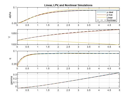
The LPV simulations are very close to the nonlinear simulation, confirming that the LPV model of the airframe is an effective surrogate and that the gain-scheduled LPV controller is performing well. As expected, the LPV simulation using the true parameter trajectory is slightly more accurate than its surrogate using p_ideal.