ltvss

Linear time-varying state-space model

Since R2023a

Description

Use ltvss to represent linear state-space models whose dynamics vary with time.

You can use ltvss to create continuous-time or discrete-time linear time-varying state-space models. In continuous time, an ltvss model is described by the following state-space equations.

$$\begin{array}{c}E(t)\dot{x}={\delta }_0(t)+A(t)(x-x_0(t))+B(t)(u-u_0(t))\\ y(t)=y_0(t)+C(t)(x-x_0(t))+D(t)(u-u_0(t))\end{array}$$

Here, A(t), B(t), C(t), D(t), and E(t) are time-varying state-space matrices and δ₀(t), x₀(t), u₀(t), and y₀(t) are time-dependent derivative, state, input, and output offsets, respectively.

In discrete time, an ltvss model is described by the following state-space equations.

$$\begin{array}{c}{E}_k{x}_{k+1}={\delta }_{0k}+A_k(x_k-x_0{}_k)+B_k(u_k-u_0{}_k)\\ y_k=y_{0k}+C_k(x_k-x_0{}_k)+D_k(u_k-u_0{}_k)\end{array}$$

Here, the integer index k counts the number of sampling periods Ts.

You can use an ltvss object to model:

• Linear systems whose coefficients vary in time.

• Nonlinear systems operating along a specific trajectory. For an example, see LTV Model of Two-Link Robot.

• Nonlinear systems operating near steady-state conditions that change in time.

Use ltvss to construct LTV models whose dynamics are described by a MATLAB^® function (the data function). Use ssInterpolant to construct LTV models that interpolate LTI snapshots as a function of time. See LPV and LTV Models for functions and operations applicable to ltvss objects.

Creation

Syntax

ltvSys = ltvss(DataFcn)

ltvSys = ltvss(DataFcn,ts)

ltvSys = ltvss(DataFcn,ts,tcheck)

ltvSys = ltvss(___,Name=Value)

Description

ltvSys = ltvss(DataFcn) creates a continuous-time LTV model. DataFcn is the name of or a handle to the data function, the user-defined MATLAB function that calculates the matrices and offsets for given t or k values.

ltvSys = ltvss(DataFcn,ts) creates a discrete-time LTV model with sample time ts.

ltvSys = ltvss(DataFcn,ts,tcheck) evaluates DataFcn at tcheck to determine the number of states, inputs, and outputs. By default, ltvss uses tcheck = 0.

ltvSys = ltvss(___,Name=Value) sets properties of the linear time-varying model using one or more name-value pair arguments. Use this syntax with any of the previous input-argument combinations.

Input Arguments

DataFcn — Data function

function name | function handle

User-defined MATLAB function for calculating matrices and offsets, specified as a function name (character vector or string) or a function handle. The data function must be of the following form.

• Continuous time — $$[A,B,C,D,E,{\delta }_0,x_0,u_0,y_0,Delays]=f(t)$$

• Discrete time — $$[A,B,C,D,E,{\delta }_0,x_0,u_0,y_0,Delays]=f(k)$$

The Delay argument is a structure with fields Input and Output specifying the delays in input and output channels, respectively. (since R2024a)

For more information about defining a data function, see Data Function.

This input sets the value of property DataFunction.

ts — Sample time

scalar

Sample time, specified as a scalar. For more information, see the Ts property.

tcheck — Time test value

scalar

Test value for time, specified as a scalar. The object evaluates DataFcn at tcheck to check if it is valid and to obtain the number of states, inputs, and outputs. By default, ltvss uses tcheck = 0.

Properties

DataFunction — Data function

[] (default) | function handle

Data function for calculating the model data, specified as a function handle. The data function must be of the following form.

• Continuous time

  [A,B,C,D,E,dx0,x0,u0,y0,Delay] = DataFcn(t)

• Discrete time

  [A,B,C,D,E,dx0,x0,u0,y0,Delay] = DataFcn(k)

  Here, the input k is an integer index that counts the number of sampling periods Ts. The absolute time is given by t = k*Ts.

To pass additional input arguments, use an anonymous function as follows.

DataFcn = @(t) myFunction(t,arg1,arg2,...)

You can set all output arguments except A, B, C, D to [] when absent for t values.

For more information, see Data Function.

StateName — State names

' ' (default) | character vector | cell array of character vectors

State names, specified as one of the following:

• Character vector — For first-order models, for example, 'velocity'.

• Cell array of character vectors — For models with two or more states.

StateName is empty ' ' for all states by default.

StatePath — State path

' ' (default) | character vector | cell array of character vectors

State path to facilitate state block path management in linearization, specified as one of the following:

• Character vector — For first-order models

• Cell array of character vectors — For models with two or more states

StatePath is empty ' ' for all states by default.

StateUnit — State units

' ' (default) | character vector | cell array of character vectors

State units, specified as one of the following:

• Character vector — For first-order models, for example, 'm/s'

• Cell array of character vectors — For models with two or more states

Use StateUnit to keep track of the units of each state. StateUnit has no effect on system behavior. StateUnit is empty ' ' for all states by default.

Ts — Sample time

0 (default) | positive scalar | -1

Sample time, specified as:

• 0 for continuous-time systems.

• A positive scalar representing the sampling period of a discrete-time system. Specify Ts in the time unit specified by the TimeUnit property.

• -1 for a discrete-time system with an unspecified sample time.

Note

Changing Ts does not discretize or resample the model. To convert between continuous-time and discrete-time representations, use c2d and d2c. To change the sample time of a discrete-time system, use d2d.

TimeUnit — Time variable units

'seconds' (default) | 'nanoseconds' | 'microseconds' | 'milliseconds' | 'minutes' | 'hours' | 'days' | 'weeks' | 'months' | 'years' | ...

Time variable units, specified as one of the following:

• 'nanoseconds'

• 'microseconds'

• 'milliseconds'

• 'seconds'

• 'minutes'

• 'hours'

• 'days'

• 'weeks'

• 'months'

• 'years'

Changing TimeUnit has no effect on other properties, but changes the overall system behavior. Use chgTimeUnit to convert between time units without modifying system behavior.

InputName — Input channel names

'' (default) | character vector | cell array of character vectors

Input channel names, specified as one of the following:

• A character vector, for single-input models.

• A cell array of character vectors, for multi-input models.

• '', no names specified, for any input channels.

Alternatively, you can assign input names for multi-input models using automatic vector expansion. For example, if sys is a two-input model, enter the following:

sys.InputName = 'controls';

The input names automatically expand to {'controls(1)';'controls(2)'}.

You can use the shorthand notation u to refer to the InputName property. For example, sys.u is equivalent to sys.InputName.

Use InputName to:

• Identify channels on model display and plots.

• Extract subsystems of MIMO systems.

• Specify connection points when interconnecting models.

InputUnit — Input channel units

'' (default) | character vector | cell array of character vectors

Input channel units, specified as one of the following:

• A character vector, for single-input models.

• A cell array of character vectors, for multi-input models.

• '', no units specified, for any input channels.

Use InputUnit to specify input signal units. InputUnit has no effect on system behavior.

InputGroup — Input channel groups

structure

Input channel groups, specified as a structure. Use InputGroup to assign the input channels of MIMO systems into groups and refer to each group by name. The field names of InputGroup are the group names and the field values are the input channels of each group. For example, enter the following to create input groups named controls and noise that include input channels 1 and 2, and 3 and 5, respectively.

sys.InputGroup.controls = [1 2];
sys.InputGroup.noise = [3 5];

You can then extract the subsystem from the controls inputs to all outputs using the following.

sys(:,'controls')

By default, InputGroup is a structure with no fields.

OutputName — Output channel names

'' (default) | character vector | cell array of character vectors

Output channel names, specified as one of the following:

• A character vector, for single-output models.

• A cell array of character vectors, for multi-output models.

• '', no names specified, for any output channels.

Alternatively, you can assign output names for multi-output models using automatic vector expansion. For example, if sys is a two-output model, enter the following.

sys.OutputName = 'measurements';

The output names automatically expand to {'measurements(1)';'measurements(2)'}.

You can also use the shorthand notation y to refer to the OutputName property. For example, sys.y is equivalent to sys.OutputName.

Use OutputName to:

• Identify channels on model display and plots.

• Extract subsystems of MIMO systems.

• Specify connection points when interconnecting models.

OutputUnit — Output channel units

'' (default) | character vector | cell array of character vectors

Output channel units, specified as one of the following:

• A character vector, for single-output models.

• A cell array of character vectors, for multi-output models.

• '', no units specified, for any output channels.

Use OutputUnit to specify output signal units. OutputUnit has no effect on system behavior.

OutputGroup — Output channel groups

structure

Output channel groups, specified as a structure. Use OutputGroupto assign the output channels of MIMO systems into groups and refer to each group by name. The field names of OutputGroup are the group names and the field values are the output channels of each group. For example, create output groups named temperature and measurement that include output channels 1, and 3 and 5, respectively.

sys.OutputGroup.temperature = [1];
sys.OutputGroup.measurement = [3 5];

You can then extract the subsystem from all inputs to the measurement outputs using the following.

sys('measurement',:)

By default, OutputGroup is a structure with no fields.

Name — System name

'' (default) | character vector

System name, specified as a character vector. For example, 'system_1'.

Notes — User-specified text

{} (default) | character vector | cell array of character vectors

User-specified text that you want to associate with the system, specified as a character vector or cell array of character vectors. For example, 'System is MIMO'.

UserData — User-specified data

[] (default) | any MATLAB data type

User-specified data that you want to associate with the system, specified as any MATLAB data type.

Object Functions

Sampling and Interpolation

sample	(Not recommended) Sample linear parameter-varying or time-varying dynamics
ssInterpolant	Build gridded LTV or LPV model from state-space data

Time Response Simulation

step	Step response of dynamic system
impulse	Impulse response plot of dynamic system; impulse response data
lsim	Plot simulated time response of dynamic system to arbitrary inputs; simulated response data
initial	System response to initial states of state-space model

Model Interconnection

feedback	Feedback connection of multiple models
connect	Block diagram interconnections of dynamic systems
series	Series connection of two models
parallel	Parallel connection of two models
lft	Generalized feedback interconnection of two models (Redheffer star product)

Model Transformation

c2d	Convert model from continuous to discrete time
d2c	Convert model from discrete to continuous time
d2d	Resample discrete-time model
xperm	Reorder states in state-space models
sminreal	Eliminates structurally disconnected states, delays, and blocks

Examples

Continuous-Time Linear Time-Varying Model

Create a continuous-time SISO linear time-varying model.

This example uses a first-order model. The matrices and offsets are given by:

$\mathit{A}=-\left(1+0.5\sin \left(\mathit{t}\right)\right)$, $\mathit{B}=1$, $\mathit{C}=1$, $\mathit{D}=0$,

${\mathit{y}}_0=0.1\sin \left(5\mathit{t}\right)$.

These matrices and offsets are defined in the ltvssDataFcn.m data function provided with this example.

Create an LTV model.

ltvSys = ltvss(@ltvssDataFcn)

Continuous-time state-space LTV model with 1 outputs, 1 inputs, and 1 states.

View the data function.

type ltvssDataFcn.m

function [A,B,C,D,E,dx0,x0,u0,y0,Delays] = ltvssDataFcn(t)
% SISO, first order
A = -(1+0.5*sin(t));
B = 1;
C = 1;
D = 0;
E = [];
dx0 = [];
x0 = [];
u0 = [];
y0 = 0.1*sin(5*t);
Delays = [];

Discrete-Time Linear Time-Varying Model

Create a discrete-time linear time-varying model.

This example uses a model with the matrices and offsets defined as:

$$\mathit{A}=\sin \left(0.1\mathit{k}\right),\mathit{B}=1,\mathit{C}=1,\mathit{D}=0$$

$${\mathit{y}}_0=0.1\sin \left(\mathit{k}\right)$$

These matrices and offsets are defined in the ltvFcnDiscrete.m data function provided with this example.

Specify the properties and create an LTV model.

Ts = 0.01;
DataFcn = @ltvFcnDiscrete;
ltvSys = ltvss(DataFcn,Ts)

Discrete-time state-space LTV model with 1 outputs, 1 inputs, and 1 states.

You can set additional properties of the model using dot notation

ltvSys.InputName = 'u';
ltvSys.OutputName = 'y';

View the data function.

type ltvFcnDiscrete.m

function [A,B,C,D,E,dx0,x0,u0,y0,Delays] = ltvFcnDiscrete(k)

A = sin(0.1*k);
B = 1;
C = 1;
D = 0;
E = [];
dx0 = [];
x0 = [];
u0 = [];
y0 = 0.1*sin(k);
Delays = [];

Time Response of Linear Time-Varying Models

For this example, ltvssDataFcn.m defines the matrices and offsets of a MIMO system.

Create an LTV model.

ltvSys = ltvss(@ltvssDataFcn);

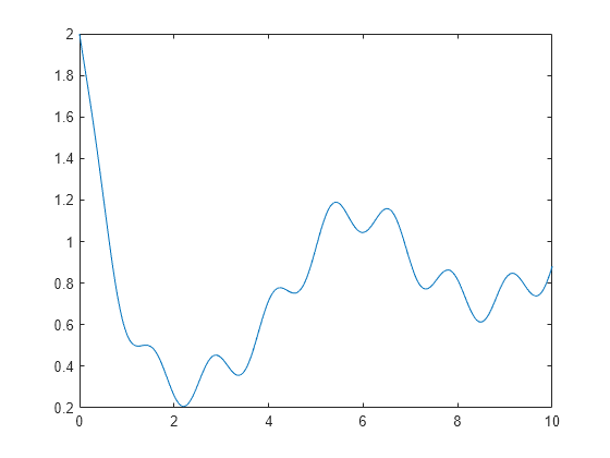
Simulate the response of this model to an arbitrary input from t = 0 to t = 10 seconds.

t = (0:.01:10)';
u = sin(0.2*t);
x0 = 2;

Simulate and plot the response.

[y,~,x] = lsim(ltvSys,u,t,x0);
plot(t,y)

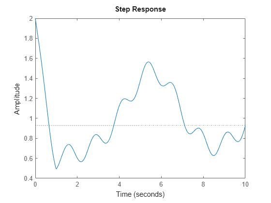
Now, simulate the model to step and impulse responses.

Create an option set using RespConfig to specify initial offset, and state values.

respOpt = RespConfig(InitialState=x0,Delay=1);

Compute the step response.

step(ltvSys,t,respOpt)

Compute the impulse response.

impulse(ltvSys,t,respOpt)

View the data function.

type ltvssDataFcn.m

function [A,B,C,D,E,dx0,x0,u0,y0,Delays] = ltvssDataFcn(t)
% SISO, first order
A = -(1+0.5*sin(t));
B = 1;
C = 1;
D = 0;
E = [];
dx0 = [];
x0 = [];
u0 = [];
y0 = 0.1*sin(5*t);
Delays = [];

Create LTV Model with Fixed and Varying Delays

Since R2024a

This example shows how to create a linear time-varying model containing fixed and varying input and output delays.

This example uses a model with the matrices, offsets, and delays defined in this data function.

function [A,B,C,D,E,dx0,x0,u0,y0,Delays] = ltvDataFcnDelay(t)
    A = [-2 1;1 -0.5*(2+sin(10*t))];
    B = [1 cos(t);sin(5*t) 0];
    C = [1,2*cos(3*t);-1 3;sqrt(t) 0];
    D = [0 0;-1 1;0 0.5*sin(t)];
    E = [];
    dx0 = [cos(10*t)/(1+0.1*t);0];
    x0 = [0;sqrt(t)/(1+0.1*t)];
    u0 = [sin(10*t);1];
    y0 = [1/(1+t);-1;cos(3*t)];
    Delays.Input = [NaN;abs(cos(0.3*t))];
    Delays.Output = [1.7;NaN;abs(sin(0.5*t))];
end

The delays argument is a structure with fields Input and Output specifying the delays corresponding input and output channels, respectively. This data function defines the delays as follows:

• No delay at all times in the first input channel and a varying delay of $\cos \left(0.3\mathit{t}\right)$ s in the second input channel.

• Fixed delay of 1.7 s in the first output channel, no delay in the second output channel, and a varying delay of $\sin \left(0.5\mathit{t}\right)$ s in the third output channel.

Create the LTV model.

ltvsysD = ltvss(@ltvDataFcnDelay)

Continuous-time state-space LTV model with 3 outputs, 2 inputs, and 2 states.
Model Properties

The software manages and propagates specified delays when you perform operations such as sampling.

Sample the model at two values of time.

t = [3,5];
sys = psample(ltvsysD,t)

sys(:,:,1,1) [Time=3] =
 
  A = 
           x1      x2
   x1      -2       1
   x2       1  -0.506
 
  B = 
           u1      u2
   x1       1   -0.99
   x2  0.6503       0
 
  C = 
           x1      x2
   y1       1  -1.822
   y2      -1       3
   y3   1.732       0
 
  D = 
            u1       u2
   y1        0        0
   y2       -1        1
   y3        0  0.07056
 
  Input delays (seconds): 0  0.622 
  Output delays (seconds): 1.7  0  0.997 
 

sys(:,:,1,2) [Time=5] =
 
  A = 
            x1       x2
   x1       -2        1
   x2        1  -0.8688
 
  B = 
            u1       u2
   x1        1   0.2837
   x2  -0.1324        0
 
  C = 
           x1      x2
   y1       1  -1.519
   y2      -1       3
   y3   2.236       0
 
  D = 
            u1       u2
   y1        0        0
   y2       -1        1
   y3        0  -0.4795
 
  Input delays (seconds): 0  0.0707 
  Output delays (seconds): 1.7  0  0.598 
 
1x2 array of continuous-time state-space models.
Model Properties

The sampled LTV model contains fixed delays and delays varying with time as defined in the data function.

Version History

Introduced in R2023a

R2024a: Data Function: Support for specifying input and output delays

Use the Delay argument of the data function to specify fixed or varying delays. The Delay argument is a structure with fields Input and Output specifying the delays in input and output channels, respectively. Set Delay.Input and Delay.Output to vectors with length equal to the number of input and output channels, respectively. To indicate the absence of delay in a particular channel at all times, set the corresponding value in the vector to NaN. For example, for a three-input system, Delay.Input = [0.1 NaN sin(0.2*t)] defines a fixed delay in the first input channel, no delay in the second channel, and a varying delay in the third input channel. For more information about the data function, see Data Function