Control Design for Spinning Disks
This example shows how to design a gain-scheduled controller for a mechanical system consisting of coupled spinning disks described in [1].
Coupled Spinning Disks
A pair of rotating disks is shown in this figure. The slotted disks rotate at rates of rad/s and rad/s. The disks contain masses and , which can move in the horizontal plane and slide radially. The two masses are connected by a wire, coupler, and pulley system that can transmit force in both compression and tension. This coupling system acts as a spring with spring constant , and friction due to the sliding motion of each mass is modeled by a damping coefficient .
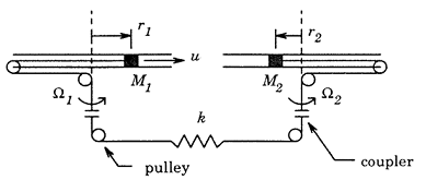
The goal is to control the positions of the two masses: for mass and for . The control input is a radial force acting on mass and radial disturbance forces and act on each mass. The equations of motions are as follows.
Here:
= 1 kg and is the mass of the sliding mass in disk 1.
= 2 kg and is the mass of the sliding mass in disk 2.
= 1 kg/s and is the damping coefficient due to friction.
= 200 N/m is the spring constant of mass coupling system.
is the position of the sliding mass relative to the center of disk 1 (m).
is the position of the sliding mass relative to the center of disk 2 (m).
is the rotational rate of disk 1 (rad/s).
is the rotational rate of disk 2 (rad/s).
is the control force acting radially on mass (N).
and are the disturbance forces acting radially on and , respectively (N).
The rotational rates of the spinning disks are allowed to vary in the ranges and (in rad/s). These rates are not known in advance but are measured and available for control design. The objective of the control design is to command the radial position of mass . Note that the control input is applied to mass and is transmitted to mass through the disk coupling system.
LPV Model
The equations of motions are linear except for the rates and . Choosing , , , and as scheduling parameters, you obtain the following LPV model of the overall system.
Here, the state vector .
To create this LPV model, write a function disksGFCN that computes the , , matrices as a function of the scheduling parameters . To see the code for this function, see the disksGFCN.m file or enter type disksGFCN at the command line.
Define system parameters.
m1 = 1;
m2 = 0.5;
k = 200;
b = 1;
Define the LPV system.
fh = @(t,p) disksGFCN(t,p,m1,m2,k,b);
G = lpvss(["p1","p2"],fh);
Gain-Scheduled H2 Control Design
Design a gain-scheduled -optimal controller. First, design an -optimal controller at each point on a grid of (,) values. For fixed rotational rates, such controllers minimize the closed-loop norm from disturbance to error for the weighted interconnection. For appropriately selected weights, this interconnection defines the desired performance of the control law. The controller takes in the reference and measurement and generates the command .
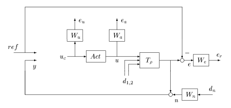
Define the weights and build an LPV model of this interconnection.
% Add input/output names to plant
G.InputName = {'u'; 'f1'; 'f2'};
G.OutputName = 'Gy';

% Actuator model
act = ss(-100,100,1,0);
act.InputName = 'uc';
act.OutputName = 'u';

% Weight: Control Command
Wu = ss(1/50);
Wu.InputName = 'uc';
Wu.OutputName = 'eu';

% Weight: Actuator Output
Wa = ss(0.00001);
Wa.InputName = 'u';
Wa.OutputName = 'ea';

% Weight: Tracking Error
We = tf(2,[1 0.04]);
We.InputName = 'e';
We.OutputName = 'er';

% Weight: Noise
Wn = tf([1,0.4],[0.01 400]);
Wn.InputName = 'dn';
Wn.OutputName = 'n';

% Form synthesis interconnection
sum1 = sumblk('y = Gy + n');
sum2 = sumblk('e = Gy - r');
IC = connect(G,act,Wu,Wa,We,Wn,sum1,sum2,{'r','f1','f2','dn','uc'},...
     {'eu','ea','er','r','y'});
Construct a grid of (,) values and compute the -optimal controller at each grid point.
p1 = linspace(0,9,3);
p2 = linspace(0,25,3);
[p1,p2] = ndgrid(p1,p2);
Sample IC at grid points and design -optimal controllers.
nmeas = 2;   % # of measurements
ncon = 1;    % # of controls
ICs = sample(IC,[],p1,p2);
Ks = ss( zeros([ncon nmeas size(p1)]) );
for i=1:numel(p1)
   Ks(:,:,i) = h2syn(ICs(:,:,i),nmeas,ncon);
end
Use ssInterpolant to create a gain-scheduled controller that linearly interpolates these controllers between grid points. This approach is valid when the rotational rates vary slowly. Alternative LPV methods for rapid changes are described in [1].
Ks.SamplingGrid = struct('p1',p1,'p2',p2);
Klpv = ssInterpolant(Ks,[]);
Klpv.InputName = {'r','Gy'};
Klpv.OutputName = {'uc'};
LTI Performance Evaluation
Evaluate the gain-scheduled controller for fixed rotation rates using a finer grid than for the controller design.
Form closed-loop system from [r;f1;f2] to Gy.
CL = connect(G,act,Klpv,{'r','f1','f2'},{'Gy'});Evaluate open and closed-loop on a finer grid of points.
p1 = linspace(0,9,5);
p2 = linspace(0,25,5);
[p1,p2] = ndgrid(p1,p2);
Gs = sample(G,[],p1,p2);
CLs = sample(CL,[],p1,p2);
The controller achieves good tracking with minimal overshoot, approximately 2.5 s settling time, and less than 3% steady-state tracking error. Furthermore, the disturbances have minimal effect.
step(CLs,5)
grid on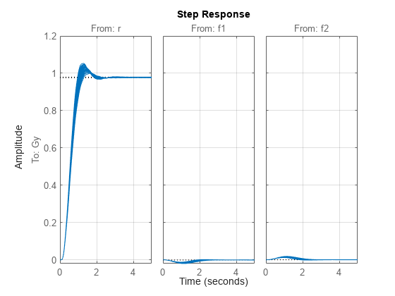
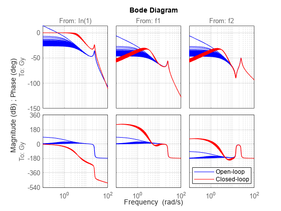
The closed-loop Bode response from r to Gy has a DC gain near one with a bandwidth near 3 rad/s. It shows good disturbance attenuation below 1 rad/s compared to the open loop.
bode(Gs,"b",CLs,"r",{0.1,100})
legend("Open-loop","Closed-loop","Location","best")
grid minor
LPV Performance Evaluation
Finally, evaluate the gain-scheduled controller with a time-domain simulation with time-varying rotation rates. The parameters vary in time as follows:
, .
The reference signal is a unit step and the disturbances are set to
, .
Define the inputs to the system.
t = 0:0.01:15;
u = ones(size(t));
d1 = cos(3*t)+sin(5*t)+cos(8*t);
d2 = cos(t)+sin(2*t)+cos(4*t);
Define the trajectories of the parameters.
p1 = sin(t)+1.5;
p2 = 0.5*cos(5*t)+3;
Simulate the LPV model with and without disturbances.
[y1,t1,x1] = lsim(CL,[u;d1;d2],t,[],[p1;p2]);
[y2,t2,x2] = lsim(CL,[u;0*d1;0*d2],t,[],[p1;p2]);

figure
plot(t1,y1,"b",t2,y2,"r");
grid on;
title("LPV Simulation")
ylabel("y");
legend("With disturbances","Without disturbances","Location","best")
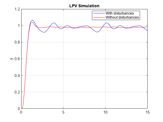
The error due to the disturbances is on the order of 5% and consists of 1–2 Hz oscillations about the disturbance-free response. This frequency range is incidentally where the LTI frequency response analysis indicates that disturbances have the greatest impact on the output signal.
Data Function
type disksGFCN.mfunction [A,B,C,D,E,dx0,x0,u0,y0,Delays] = GFCN(t,p,m1,m2,k,b)
% Matrices and offsets for LPV model of spinning disks.
% Enforce 0<=p1<=9, 0<=p2<=25
p(1) = max(0,min(p(1),9));
p(2) = max(0,min(p(2),25));
% Define state-space matrices
A = [ 0 0 1 0 ; ...
0 0 0 1 ; ...
p(1)-k/m1 -k/m1 -b/m1 0 ; ...
-k/m2 p(2)-k/m2 0 -b/m2 ];
B = [ 0 0 0 ; ...
0 0 0 ; ...
1/m1 .1/m1 0 ; ...
0 0 .1/m2 ];
C = [ 0 1 0 0];
D = [0 0 0];
E = [];
% no offsets or delays
dx0 = []; x0 = []; u0 = []; y0 = []; Delays = [];
References
[1] Wu, Fen. "Control of Linear Parameter Varying Systems," Ph.D. dissertation, Department of Mechanical Engineering, University of California at Berkeley, May 1995.