Elektrische Systeme
Erkunden Sie Beispiele, die die Modellierung, Regelung und Simulation elektrischer Systeme veranschaulichen.
Kategorien
- Elektrische Schaltkreise in Simulink und Simscape
Beispiele für elektrische Schaltkreise in Simulink® und Simscape™
- Batterien
Beispiele für Batterien
Enthaltene Beispiele
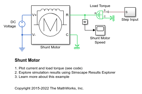
Shunt Motor
A model of a shunt motor. In a shunt motor, the field and armature windings are connected in parallel. Equivalent circuit parameters are armature resistance Ra = 110 Ohms, field resistance Rf = 2.46KOhms, and back emf coefficient Laf = 5.11. The back-emf is given by Laf*If*Ia*w, where If is the field current, Ia is the armature current, and w is the rotor speed in radians/s. The rotor inertia J is 2.2e-4kgm^2, and rotor damping B is 2.8e-6Nm/(radian/s).
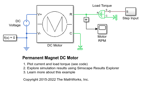
Permanentmagnet-Gleichstrommotor
Dieses Beispiel zeigt, wie Sie die Herstellerangaben zu Leerlaufdrehzahl, Leerlaufstrom und Stillstandsdrehmoment für einen Gleichstrommotor mithilfe eines Testkabelstrangs und Simscape™-Blöcken überprüfen können.
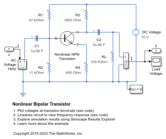
Nichtlinearer Bipolartransistor
Dieses Modell zeigt eine Implementierung eines nichtlinearen bipolaren Transistors auf der Grundlage des Ebers-Moll-Ersatzschaltbildes. R1 und R2 legen den nominalen Arbeitspunkt fest, und die Kleinsignalverstärkung wird ungefähr durch das Verhältnis R3/R4 bestimmt. Die 1uF-Entkopplungskondensatoren wurden so gewählt, dass sie bei 1 KHz eine vernachlässigbare Impedanz aufweisen. Das Modell ist für die Linearisierung konfiguriert, so dass ein Frequenzgang erstellt werden kann.
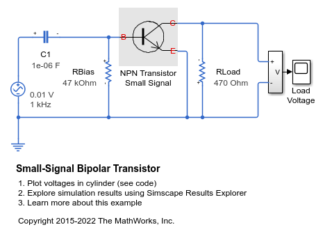
Small-Signal Bipolar Transistor
The use of a small-signal equivalent transistor model to assess performance of a common-emitter amplifier. The 47K resistor is the bias resistor required to set nominal operating point, and the 470 Ohm resistor is the load resistor. The transistor is represented by a hybrid-parameter equivalent circuit with circuit parameters h_ie (base circuit resistance), h_oe (output admittance), h_fe (forward current gain), and h_re (reverse voltage transfer ratio). Parameters set are typical for a BC107 Group B transistor. The gain is approximately given by -h_fe*470/h_ie =-47. The 1uF decoupling capacitor has been chosen to present negligible impedance at 1KHz compared to the input resistance h_ie, so the output voltage should be 47*10mV = 0.47V peak.
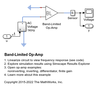
Band-Limited Op-Amp
How higher fidelity or more detailed component models can be built from the Foundation library blocks. The model implements a band-limited op-amp. It includes a first-order dynamic from inputs to outputs, and gives much faster simulation than if using a device-level equivalent circuit, which would normally include multiple transistors. This model also includes the effects of input and output impedance (Rin and Rout in the circuit), but does not include nonlinear effects such as slew-rate limiting.
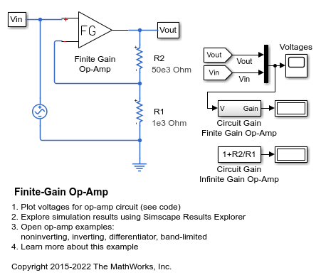
Finite-Gain Op-Amp
How higher fidelity or more detailed component models can be built from the Foundation library blocks. The Op-Amp block in the Foundation library models the ideal case whereby the gain is infinite, input impedance infinite, and output impedance zero. The Finite Gain Op-Amp block in this example has an open-loop gain of 1e5, input resistance of 100K ohms and output resistance of 10 ohms. As a result, the gain for this amplifier circuit is slightly lower than the gain that can be analytically calculated if the op-amp gain is assumed to be infinite.
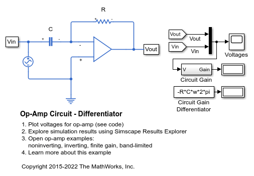
Operationsverstärkerschaltung – Differenzierer
Dieses Modell zeigt einen Differenzierer, wie er beispielsweise als Teil eines PID-Reglers verwendet werden könnte. Es veranschaulicht auch, wie bei einigen idealisierten Schaltungen Probleme bei der numerischen Simulation auftreten können. Der parasitäre Serienwiderstand des Kondensators im Modell ist auf den Standardwert von 1e-6 Ohm eingestellt. Wenn Sie den Wert auf null setzen, wird eine Warnung ausgegeben und die Simulation läuft sehr langsam. Weitere Informationen finden Sie im Benutzerhandbuch.
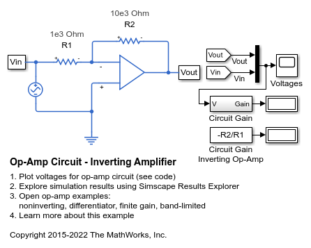
Operationsverstärkerschaltung – Invertierender Verstärker
Dieses Beispiel zeigt ein Modell einer invertierenden Standard-Operationsverstärkerschaltung. Die Verstärkung ist durch -R2/R1 gegeben. Die Spitze-Spitze-Eingangsspannung wird von 0,1 V auf 1 V Spitze-Spitze verstärkt, wenn gilt: R1=1.000 Ohm und R2=10.000 Ohm. Der Block „Op-Amp“ implementiert ein ideales (d. h. unendlich verstärktes) Gerät. Daher wird diese Verstärkung unabhängig von der Ausgangslast erreicht.
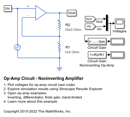
Operationsverstärkerschaltung – Nicht invertierender Verstärker
Dieses Modell zeigt eine nicht invertierende Operationsverstärkerschaltung. Die Verstärkung wird durch 1+R2/R1 angegeben, und wenn die Werte R1=1.000 Ohm und R2=10.000 Ohm festgelegt sind, wird die Spitze-Spitze-Eingangsspannung von 0,1 V auf 1,1 V Spitze-Spitze verstärkt. Da der Block „Op-Amp“ ein ideales (d. h. unendlich verstärktes) Gerät implementiert, wird diese Verstärkung unabhängig von der Ausgangslast erreicht.
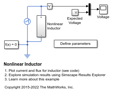
Nonlinear Inductor
An implementation of a nonlinear inductor where inductance depends on current. A tanh function defines the nonlinear flux-current relationship. The flux saturates for large currents, which can occur, for example, in iron core inductors.
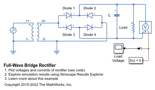
Vollwellen-Brückengleichrichter
Dieses Beispiel zeigt, wie man einen Kondensator für eine bestimmte Last in einem Transformator dimensioniert, der 120 V Wechselspannung in 12 V Gleichspannung umwandelt. Das System wird als idealer Wechselstromtransformator mit Vollwellen-Brückengleichrichter modelliert.
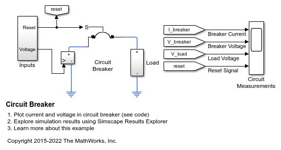
Circuit Breaker
Model a circuit breaker. The electromechanical breaker mechanism is approximated with a first-order time constant, and it is assumed that the mechanical force is proportional to load current. This simple representation is suitable for use in a larger model of a complete system. When the 20V supply is applied at one second, it results in a current that exceeds the circuit breaker current rating, and hence the breaker trips. The reset is then pressed at three seconds, and the voltage is ramped up. The breaker then trips just beyond the circuit breaker current rating.
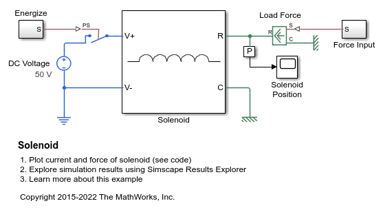
Magnetventil
In diesem Beispiel ist ein Magnetventil mit Federrückstellung dargestellt. Das Magnetventil wird als Induktivität modelliert, deren Wert L von der Kolbenposition x abhängig ist. Die elektromotorische Gegenkraft für eine mit der Zeit variierende Induktivität wird wie folgt angegeben:
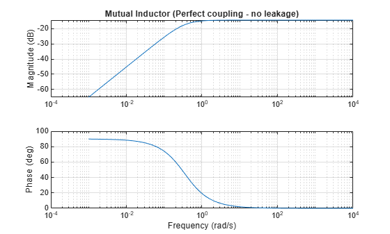
A Comparison of the Mutual Inductor and Ideal Transformer Library Blocks
The differences in behavior between the Mutual Inductor and Ideal Transformer blocks in the Simscape™ Foundation Library. These two blocks both represent the same system of electromagnetically-coupled windings but make different simplifying assumptions. It is important to understand the assumptions and how they impact model fidelity as a function of frequency. With this, you can make an informed decision about which block to use in a model of your circuit.
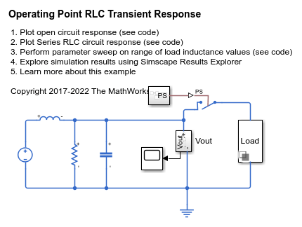
Operating Point RLC Transient Response
The response of a DC power supply connected to a series RLC load. The goal is to plot the output voltage response when a load is suddenly attached to the fully powered-up supply. This is done using a Simscape operating point.