Filter Analyzer

View, analyze, and compare filters

Since R2024a

Description

The Filter Analyzer app is an interactive tool for visualizing, analyzing, and comparing digital filters. Using the app, you can

• Import filter objects or filter coefficients. For more information, see Import Filter.

• View, analyze, and compare responses of multiple digital filters. For more information, see Analysis.

• View a list of filters in the Filters table and the details for each filter in the Filter Information table.

• Plot a new filter analysis plot in a separate display window.

• Specify filter sample rate and analysis sample rate separately.

• Save the state of the current session, including filters, displays, and analysis options, for use in a future session of the app.

You can use the filterAnalyzer command-line interface to add, remove, and update filters, displays, and analysis options.

×

Open the Filter Analyzer App

• MATLAB^® Toolstrip: On the Apps tab, under Signal Processing and Communications, click the app icon.

• MATLAB command prompt: Enter filterAnalyzer.

Examples

Analyze Filters

Design sixth-order Chebyshev Type 1 lowpass and highpass filters with normalized passband edge frequency $0.4\pi$ rad/sample and 12 dB of passband ripple. Express the designs as cascades of fourth-order transfer functions. Use Filter Analyzer to display the magnitude and phase responses of the filters.

[zl,pl,kl] = cheby1(6,12,0.4);
[bl,al] = zp2ctf(zl,pl,kl,SectionOrder=4);
[zh,ph,kh] = cheby1(6,12,0.4,"high");
[bh,ah] = zp2ctf(zh,ph,kh,SectionOrder=4);

filterAnalyzer(bl,al,bh,ah,OverlayAnalysis="phase")

Design a 30th-order FIR bandpass filter designed to filter signals sampled at 2 kHz. Specify a stopband ranging from 250 Hz to 400 Hz. Use Filter Analyzer to display the poles and zeros of the filter transfer function.

iirbp = designfilt("bandpassfir",FilterOrder=30, ...
    CutoffFrequency1=250,CutoffFrequency2=400, ...
    SampleRate=2000);

filterAnalyzer(iirbp,Analysis="polezero")

Analyze Elliptic and FIR Bandpass Filters

Design a tenth-order elliptic bandpass filter with 5 dB of passband ripple and 60 dB of stopband attenuation. Specify passband edge frequencies of $0.2\pi$ rad/sample and $0.45\pi$ rad/sample. Express the design as a cascade of fourth-order transfer functions.

[z,p,k] = ellip(5,5,60,[0.2 0.45]);
[bb,aa] = zp2ctf(z,p,k,SectionOrder=4);

Design a finite impulse response bandpass filter with 5 dB of passband ripple and asymmetric stopbands for use with signals sampled at 2 kHz.

• At lower frequencies, the stopband has 80 dB of attenuation and the transition region ranges from 500 Hz to 600 Hz.

• At higher frequencies, the stopband has 40 dB of attenuation and the transition region ranges from 750 Hz to 900 Hz.

dfir = designfilt("bandpassfir", ...
    SampleRate=2e3,PassbandRipple=5, ...
    StopbandFrequency1=500,PassbandFrequency1=600, ...
    StopbandAttenuation1=80, ...
    PassbandFrequency2=750,StopbandFrequency2=900, ...
    StopbandAttenuation2=40);

Start a Filter Analyzer session to analyze the filters. Import the filters. On the Analyzer tab, click Import Filter.

• To import the elliptic filter, select Filter Coefficients. Enter bb as the Numerator and aa as the Denominator. Choose Ellip for the Filter Name and leave the Sample Rate as Normalized. Click Import.

• To import the FIR filter, select Filter Objects, select dfir, and click Import and Close.

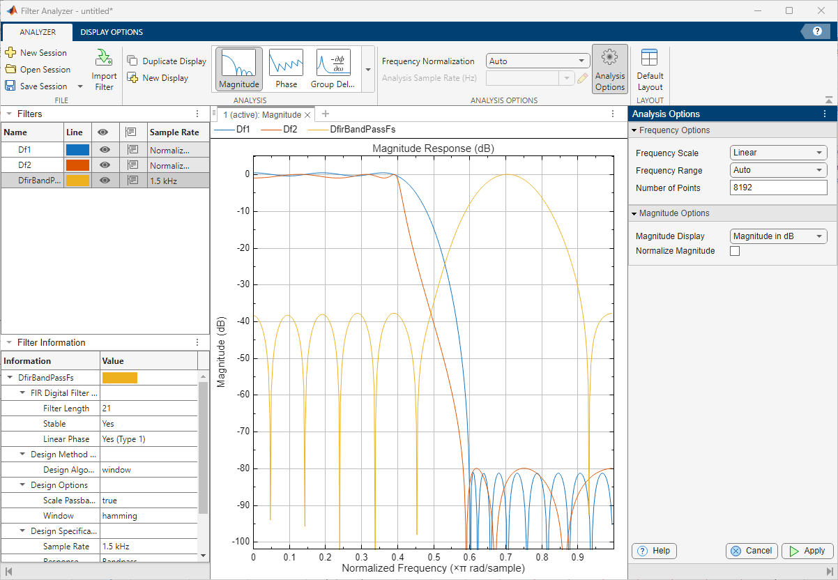
Alternatively, open Filter Analyzer by using the command-line interface. By default, the app displays magnitude responses. Only one of the filters has a sample rate, so the app displays the responses using normalized frequencies.

fa = filterAnalyzer(bb,aa,dfir,FilterNames=["ellip" "dfir"]);

Add a display and use it to plot the magnitude responses and the phase responses of the filters.

• On the Analyzer tab, click New Display.

• Expand the Analysis gallery so the Overlay Analysis section is visible and click Phase.

• Add the filters by clicking the eye icons on the Filters table.

Alternatively, use the filterAnalysisOptions, addDisplays, and showFilters functions.

opts = filterAnalysisOptions(OverlayAnalysis="phase");
addDisplays(fa,AnalysisOptions=opts)
showFilters(fa,true,FilterNames=["ellip" "dfir"])

Add another display and show the cumulative magnitude responses of the cascaded transfer functions that specify the elliptic filter.

• Click New Display to add the display and click the eye icon for the elliptic filter.

• On the Display Options tab, click CTF View ▼ and select Cumulative.

Alternatively, use the command-line interface.

addDisplays(fa,CTFAnalysisMode="cumulative")

showFilters(fa,true,FilterNames="ellip")

Add one more display and show the filter specification mask for the FIR filter.

• On the Analyzer tab, click New Display and click the eye icon for the FIR filter. The app displays the frequencies in units of Hz.

• For a digitalFilter object, the app shows the specification mask by default. To remove the mask, on the Display Options tab, click Mask ▼ and deselect Specification.

Alternatively, use the command-line interface.

addDisplays(fa)

showFilters(fa,true,FilterNames="dfir")

Related Examples

• Practical Introduction to Digital Filter Design
• Filter Design Gallery

Parameters

Filters — View and edit filter information

table

Use the Filters table to edit information about the filters under analysis.

• Name — Click this column to edit the name of the filter. You can also right-click the filter in the Filters table and select Rename.

• Line — Click this column to edit the color used to display the filter responses.

• Eye — Click this column to add the filter to the current display or to remove it.

• Cursor — Click this column to show or remove a data cursor for the filter.

• Sample Rate — Click this column to edit the sample rate for the filter.

To duplicate a filter, right-click it in the Filters table and select Duplicate.

To delete a filter from the app, right-click it in the Filters table and select Delete.

Analyzer — File, analysis, and analysis options

toolstrip tab

Import Filter — Import filter from MATLAB workspace

toolstrip button

Click Import Filter to import the filter you want to analyze. Filter Analyzer supports these filter types.

Filter Coefficients

You can use Filter Analyzer to analyze filters specified as numerator and denominator coefficients. If you specify the coefficients as the K-row matrices

$$B=\left[\begin{array}{cccc}{b}_{11}& b_{12}& \cdots & b_{1,m+1}\\ b_{21}& b_{22}& \cdots & b_{2,m+1}\\ ⋮& ⋮& \ddots & ⋮\\ b_{K1}& b_{K2}& \cdots & b_{K,m+1}\end{array}\right],A=\left[\begin{array}{cccc}{a}_{11}& a_{12}& \cdots & a_{1,n+1}\\ a_{21}& a_{22}& \cdots & a_{2,n+1}\\ ⋮& ⋮& \ddots & ⋮\\ a_{K1}& a_{K2}& \cdots & a_{K,n+1}\end{array}\right],$$

Signal Analyzer assumes you have specified the filter as a sequence of K cascaded transfer functions (CTF) such that the full transfer function of the filter is

$$H\left(z\right)=\frac{b_{11}+b_{12}{z}^{-1}+\cdots +b_{1,m+1}{z}^{-m}}{a_{11}+a_{12}{z}^{-1}+\cdots +a_{1,n+1}{z}^{-n}}\times \frac{b_{21}+b_{22}{z}^{-1}+\cdots +b_{2,m+1}{z}^{-m}}{a_{21}+a_{22}{z}^{-1}+\cdots +a_{2,n+1}{z}^{-n}}\times \cdots \times \frac{b_{K1}+b_{K2}{z}^{-1}+\cdots +b_{K,m+1}{z}^{-m}}{a_{K1}+a_{K2}{z}^{-1}+\cdots +a_{K,n+1}{z}^{-n}},$$

where m ≥ 0 is the numerator order of the filter and n ≥ 0 is the denominator order.

• If K = 1, then B and A are row vectors that specify the transfer function of an IIR filter.

• If you specify both B and A as column vectors, Filter Analyzer assumes they represent the transfer function of an IIR filter.

• If B is a scalar, Filter Analyzer assumes you specified the filter as a cascade of all-pole IIR filters with each section having a scaling gain equal to B.

• If A is a scalar, Filter Analyzer assumes you specified the filter as a cascade of FIR filters with each section having a scaling gain equal to 1/A.

Note

• To convert second-order section matrices to cascaded transfer functions, use the sos2ctf function.

• To convert a zero-pole-gain filter representation to cascaded transfer functions, use the zp2ctf function.

Coefficients and Gain

If you have a scaling gain separate from the coefficient values, you can enter it in Filter Analyzer using the Import Filter dialog box. At the command line, you can specify the coefficients and gain as a cell array of the form {B,A,g}, where B and A are as previously defined.

The gain can be a scalar overall gain or a vector of section gains.

• If the gain is a scalar, Filter Analyzer applies the value uniformly to all the cascade filter sections.

• If the gain is a vector, it must have one more element than the number of filter sections in the cascade. Filter Analyzer applies a scale value to each of the filter sections and applies the last value uniformly to all the filter sections.

If you specify the coefficient matrices and gain vector as

$$B=\left[\begin{array}{cccc}{b}_{11}& b_{12}& \cdots & b_{1,m+1}\\ b_{21}& b_{22}& \cdots & b_{2,m+1}\\ ⋮& ⋮& \ddots & ⋮\\ b_{K1}& b_{K2}& \cdots & b_{K,m+1}\end{array}\right],A=\left[\begin{array}{cccc}{a}_{11}& a_{12}& \cdots & a_{1,n+1}\\ a_{21}& a_{22}& \cdots & a_{2,n+1}\\ ⋮& ⋮& \ddots & ⋮\\ a_{K1}& a_{K2}& \cdots & a_{K,n+1}\end{array}\right],g=\left[\begin{array}{ccccc}{g}_1& g_2& \cdots & g_K& g_0\end{array}\right],$$

Signal Analyzer uses the transfer function

$$H\left(z\right)=g_0\left(g_1\frac{b_{11}+b_{12}{z}^{-1}+\cdots +b_{1,m+1}{z}^{-m}}{a_{11}+a_{12}{z}^{-1}+\cdots +a_{1,n+1}{z}^{-n}}\times g_2\frac{b_{21}+b_{22}{z}^{-1}+\cdots +b_{2,m+1}{z}^{-m}}{a_{21}+a_{22}{z}^{-1}+\cdots +a_{2,n+1}{z}^{-n}}\times \cdots \times g_K\frac{b_{K1}+b_{K2}{z}^{-1}+\cdots +b_{K,m+1}{z}^{-m}}{a_{K1}+a_{K2}{z}^{-1}+\cdots +a_{K,n+1}{z}^{-n}}\right).$$

digitalFilter Objects

You can use Filter Analyzer to analyze digitalFilter objects. Use designfilt to generate or edit digital filters based on frequency-response specifications.

Filter System Objects

If you have DSP System Toolbox™, you can use Filter Analyzer to analyze these filter System objects.

System object™
dsp.AllpassFilter
dsp.AllpoleFilter
dsp.BiquadFilter
dsp.CICCompensationDecimator
dsp.CICCompensationInterpolator
dsp.CICDecimator
dsp.CICInterpolator
dsp.CoupledAllpassFilter
dsp.Delay
dsp.Differentiator
dsp.DigitalDownConverter
dsp.DigitalUpConverter
dsp.FIRDecimator
dsp.FIRFilter
dsp.FIRHalfbandDecimator
dsp.FIRHalfbandInterpolator
dsp.FIRInterpolator
dsp.FIRRateConverter
dsp.FarrowRateConverter
dsp.FilterCascade
dsp.FourthOrderSectionFilter — Filter Analyzer does not support fixed-point arithmetic for this object
dsp.HighpassFilter
dsp.IIRFilter
dsp.IIRHalfbandDecimator
dsp.IIRHalfbandInterpolator
dsp.LowpassFilter
dsp.NotchPeakFilter — Filter Analyzer does not support fixed-point arithmetic for this System object
dsp.ParallelFilter
dsp.SOSFilter
dsp.VariableBandwidthFIRFilter
dsp.VariableBandwidthIIRFilter

Analysis — Display filter analysis

gallery

Filter Analyzer supports these analysis types. To access the options available for each analysis, use the Analysis Options button in the Analysis Options toolstrip section.

Frequency-Domain Analyses

Analysis	Icon	Options	Description
Magnitude response		Magnitude Mode: Select dB, Linear, Squared, or Zero Phase Normalize Magnitude: Toggle on or off	The frequency response is the filter transfer function evaluated at the unit circle, H(z) = H(ejω). The frequency response is in general complex-valued. You can choose to plot the magnitude of the frequency response, either in linear units or in decibels, or its magnitude squared. The zero-phase response Hr(ω) is related to the frequency response by H(ejω) = Hr(ω)ejϕ(ω), where ϕ(ω) is the continuous phase. For more information, see freqz and zerophase. If you import a filter System object, see freqz and zerophase.
Phase response		Phase Units: Select Radians or Degrees Phase Display: Select Phase or Continuous	The phase response is the frequency-dependent phase angle ϕ(ω) of the filter transfer function. For more information, see phasez, angle, and unwrap. If you import a filter System object, see phasez.
Group delay response		Group Delay Units: Select Samples or Time	The group delay is the derivative of the phase response with respect to frequency. The group delay is the average delay of the filter as a function of frequency. For more information, see grpdelay. If you import a filter System object, see grpdelay.
Phase delay response		Phase Units: Select Radians or Degrees	The phase delay is the phase response divided by the frequency. The phase delay is the time delay the filter imposes on each frequency component of the input signal. For more information, see phasedelay. If you import a filter System object, see phasedelay.
Magnitude estimate		Magnitude Mode: Select dB, Linear, or Squared Normalize Magnitude: Toggle on or off Number of Trials: Specify a number	Filter Analyzer estimates the magnitude response by filtering sinusoids with uniformly distributed random frequencies and computing the ratio of output to input. For more information, see freqrespest and freqrespopts.
Round-off noise power spectrum		Number of Trials: Specify a number	Filter Analyzer can compute the power spectral density due to the round-off noise produced by quantization errors within the filter. The result is an average over the specified number of trials. For more information, see noisepsd and noisepsdopts.

Time-Domain Analyses

Analysis	Icon	Options	Description
Impulse response		Specify Length: Select Auto or User-defined	The impulse response is the response of the filter to a unit impulse. The transfer function is the Fourier transform of the impulse response. For more information, see impz. If you import a filter System object, see impz.
Step response		Specify Length: Select Auto or User-defined	The step response is the response of the filter to a step input. The step response is the cumulative sum of the impulse response. For more information, see stepz. If you import a filter System object, see stepz.

Other Analyses

Analysis	Icon	Options	Description
Pole-zero plot		N/A	The pole-zero plot shows the poles and zeros of the filter transfer function on the z-plane. Filter Analyzer uses the symbol o to denote a zero and the symbol x to denote a pole. For more information, see zplane. If you import a filter System object, see zplane.
Filter coefficients		Coefficients Format: Select Decimal, Hexadecimal, or Binary	The coefficients depend on the filter structure (cascaded transfer functions, direct-form, lattice). For filters specified as cascaded transfer functions, Filter Analyzer displays the numerator coefficients, denominator coefficients, and gain of each section of the cascade separately. You must have a Fixed-Point Designer™ license to use the Binary option.
Filter information		N/A	The filter information includes the structure, phase, stability, and implementation cost of the filter.

Analysis Options — Frequency display and sample rates

tab section

Frequency Normalization

In Filter Analyzer, you can display filter responses using normalized frequencies or in terms of a sample rate of your choice. To select how to display frequencies, on the Analysis Options section of the Analyzer tab, click Frequency Normalization.

• Auto — If some filters do not have a sample rate, analyze filter responses using normalized frequencies measured in rad/sample. If all filters have a sample rate, analyze filter responses using cyclical frequencies measured in Hz.

• Normalized — Analyze filter responses using normalized frequencies measured in rad/sample.

• Unnormalized — Analyze filter responses using cyclical frequencies measured in Hz.

Analysis Sample Rate

You can choose a reference sample rate to compare the filters plotted in a display by entering a value in the Analysis Options section of the Analyzer tab. You can also choose the highest sample rate among all the filters in the display by selecting Max. To edit the sample rate units, click the pencil icon.

Analysis Options

These options are available for all frequency-domain analyses:

• Frequency Scale — To display responses in linear frequency scale, select Linear. To use a logarithmic frequency scale, select Log.

• Frequency Range — To display responses over positive frequencies only, select One Sided. To display responses over the whole frequency range, select Two Sided. To display responses over the whole frequency range centered at zero, select Centered. To display responses over a custom range of frequencies, select User-defined.

• Number of Points — Select the number of discrete Fourier transform points you want to use to display frequency-domain responses.

For a list of options available with each analysis type, see Analysis.

Display Options — Annotations and advanced settings

toolstrip tab

View — Legend, grid, cursors, masks

tab section

Filter Analyzer supports these display options:

• Legend — Click the button to show or hide legends in the active display or in all displays.

• Grid — Click the button to show or hide the grid in the active display or in all displays.

• Hide Cursors — Click the button to hide the cursors in the active display or in all displays. To show the cursor corresponding to a given filter, click in the cursor column of a signal in the Filters table.

• Mask — Click the button to show or hide the spectral mask in the active display. You can use a standard filter specification mask or you can define your own.

  Specify a custom mask as a set of frequencies and a corresponding set of values. To specify your selection, click User Settings. You can use normalized frequencies or express frequencies in units of Hz, kHz, MHz, or GHz. You can specify values for the magnitude of interest, the square of the magnitude, or the magnitude expressed in dB. The frequencies and the values must be finite.

  Note

  Standard specification masks are available only for filters with design metadata. To include metadata in your design, use a digitalFilter object or a filter System object.

CTF View — Visualize cascaded transfer functions

tab section

If you specify a filter as a cascade of transfer functions, you can choose the way that Filter Analyzer displays section-by-section responses. This option applies only for displays with one filter. In the Display Options tab, click CTF View to toggle between displaying the overall response and displaying the responses section by section. Click CTF View ▼ to select one of these options:

• Individual — Show filter responses of individual sections.

• Cumulative — Show filter responses of cumulative sections.

• User-defined — Show filter responses of selected sections or combinations of sections. To specify your selection, click User Settings and use a cell array.

  For example, {[1 2 3],[4 5 6]} directs the app to display responses for a cascade of sections 1, 2, and 3 and a cascade of sections 4, 5, and 6.

Programmatic Use

filterAnalyzer(filt1,...,filtn)

filterAnalyzer(filt1,...,filtn) plots the responses of the specified filters in the Filter Analyzer app.

• If Filter Analyzer is not open, this syntax opens the app and plots the responses.

• If Filter Analyzer is open, this syntax plots the responses in a new display in the app.

Specify input filters as coefficient matrices, cell arrays, digitalFilter objects, or System objects. For more information, see Import Filter.

filterAnalyzer(filt1,...,filtn,Name=Value)

filterAnalyzer(filt1,...,filtn,Name=Value) specifies nondefault options using one or more name-value arguments.

filterAnalyzer(filename)

filterAnalyzer(filename) opens a Filter Analyzer session stored in the MAT-file called filename. If Filter Analyzer is already open, this syntax replaces the current app session with the new session.

filterAnalyzer(filename,"append")

filterAnalyzer(filename,"append") appends the filters stored in the MAT-file called filename to the current Filter Analyzer session. If Filter Analyzer is not open, this syntax is equivalent to the previous syntax.

[fa,dispnums] = filterAnalyzer(___)

[fa,dispnums] = filterAnalyzer(___) returns a handle object for the Filter Analyzer and the numbers corresponding to the newly added displays. You can also obtain the handle fa by typing fa = getFilterAnalyzerHandle at the command line.

Version History

Introduced in R2024a