dsp.SOSFilter
Implement cascade of second order section filters
Description
The dsp.SOSFilter
System object™ implements an IIR filter structure using second-order sections (SOS).
To implement an IIR filter structure using SOS:
Create the
dsp.SOSFilterobject and set its properties.Call the object with arguments, as if it were a function.
To learn more about how System objects work, see What Are System Objects?
This object supports C/C++ code generation and SIMD code generation under certain conditions. This object also supports code generation for ARM® Cortex®-M and ARM Cortex-A processors. For more information, see Code Generation.
Creation
Syntax
Description
sos = dsp.SOSFiltersos, which independently filters each channel (column)
of the input over time using a specified biquadratic structure.
sos = dsp.SOSFilter(num,den)Numerator property set
to num and the Denominator property set to
den.
sos = dsp.SOSFilter(___,SampleRate=Value)"normalized". (since R2026a)
To specify an input sample rate of 22050 Hz, set
SampleRate to 22050. To specify the input sample rate in normalized
units, set SampleRate to "normalized". (since R2026a)
sos = dsp.SOSFilter(___,PropertyName,Value)
Example: sos = dsp.SOSFilter('CoefficientSource','Input
port')
Properties
Usage
Description
Input Arguments
Output Arguments
Object Functions
To use an object function, specify the
System object as the first input argument. For
example, to release system resources of a System object named obj, use
this syntax:
release(obj)
Examples
Lowpass filter a noisy sinusoidal signal using the dsp.SOSFilter System object. Visualize the original and filtered signals using a spectrum analyzer.
Input Signal
The input signal is a sinusoidal signal with two tones, one at 1 kHz and the other at 3 kHz. The sampling frequency is 8 kHz.
f1 = 1000;
f2 = 3000;
Fs = 8000;
sine = dsp.SineWave(Frequency=[f1,f2],...
    SampleRate=Fs,...
    SamplesPerFrame=1024);
Create Biquad SOS Filter
Design a 10th-order lowpass Butterworth IIR filter with a cutoff frequency of 2 kHz. The numerator and denominator coefficients are extracted from the designed SOS matrix.
Fcutoff = 2000;
[z,p,k] = butter(10,Fcutoff/(Fs/2));
[s, g]  = zp2sos(z,p,k);
[num,den] = sos2ctf(s);

sosFilter = dsp.SOSFilter(num,den,...
    ScaleValues=g)
sosFilter =
dsp.SOSFilter with properties:
Structure: 'Direct form II transposed'
CoefficientSource: 'Property'
Numerator: [5×3 double]
Denominator: [5×3 double]
HasScaleValues: true
ScaleValues: [0.0029 1 1 1 1 1]
Show all properties
Visualize the frequency response of the designed SOS filter.
freqz(sosFilter,[],8000)

Streaming
Add zero-mean white Gaussian noise with a standard deviation of 0.1 to the sum of sine waves. Filter the noisy sinusoidal signal with the designed SOS filter.
While running the simulation, the spectrum analyzer shows that the high-frequency tone above 2 kHz in the source signal is attenuated. The resulting signal maintains the peak at 1 kHz because it falls in the passband of the lowpass filter.
SA = spectrumAnalyzer(...
        PlotAsTwoSidedSpectrum=false, ...
        SampleRate=Fs, ...
        ShowLegend=true,...
        YLimits=[-200 100],...
        ChannelNames={'Input signal','Filtered signal'});

    % Stream processing loop
for k = 1:100
    input = sum(sine(),2) + 0.1.*randn(sine.SamplesPerFrame,1);
    filteredOutput = sosFilter(input);
    SA(input,filteredOutput);
end

Design a lowpass biquadratic SOS filter with time-varying coefficients. Visualize the magnitude response of the filter using a dynamic filter visualizer.
dfv = dsp.DynamicFilterVisualizer('YLimits',[-120 10])dfv =
dsp.DynamicFilterVisualizer handle with properties:
NumFrequencyPoints: 2048
NormalizedFrequency: 0
SampleRate: 44100
FrequencyRange: [0 22050]
XScale: 'Linear'
MagnitudeDisplay: 'Magnitude (dB)'
PlotAsMagnitudePhase: 0
AxesScaling: 'Manual'
Show all properties
Create a dsp.SOSFilter object.
sosfilt = dsp.SOSFilter
sosfilt =
  dsp.SOSFilter with properties:

            Structure: 'Direct form II transposed'
    CoefficientSource: 'Property'
            Numerator: [0.0975 0.1950 0.0975]
          Denominator: [1 -0.9428 0.3333]
       HasScaleValues: false

  Show all properties
Use the maxflat function to design a lowpass maximally flat filter. Set the numerator and denominator order of the filter to 2 since the SOS filter is biquadratic. Vary the cutoff frequency in 0.001 increments and design the filter for each increment. Pass the computed coefficients to the SOS filter. Visualize the time-varying magnitude response of the SOS filter using the dsp.DynamicFilterVisualizer object.
for Wn = 0.1:0.001:0.6
 [b,a] = maxflat(2,2,Wn);
 sosfilt.Numerator = b;
 sosfilt.Denominator = a;
 dfv(sosfilt)
end

Design a peak filter of order 14 and a center frequency at 0.2 rad/s using the designNotchPeakIIR function. Output scale values by setting the HasScaleValues property to true.
[b,a,sv] = designNotchPeakIIR(FilterOrder=14, CenterFrequency=0.2,...
    HasScaleValues=true)
b = 7×3
1.0000 2.0000 1.0000
1.0000 -2.0000 1.0000
1.0000 2.0000 1.0000
1.0000 -2.0000 1.0000
1.0000 2.0000 1.0000
1.0000 -2.0000 1.0000
1.0000 0 -1.0000
a = 7×3

    1.0000   -1.4026    0.9374
    1.0000   -1.7004    0.9549
    1.0000   -1.3637    0.8373
    1.0000   -1.6111    0.8736
    1.0000   -1.3788    0.7823
    1.0000   -1.5195    0.8103
    1.0000   -1.4366    0.7757
sv = 8×1

    0.1220
    0.1220
    0.1166
    0.1166
    0.1133
    0.1133
    0.1122
    1.0000
Assign the filter design coefficients to a dsp.SOSFilter object.
peakFilter = dsp.SOSFilter(b,a,ScaleValues=sv)
peakFilter =
  dsp.SOSFilter with properties:

            Structure: 'Direct form II transposed'
    CoefficientSource: 'Property'
            Numerator: [7×3 double]
          Denominator: [7×3 double]
       HasScaleValues: true
          ScaleValues: [8×1 double]

  Show all properties
Create a dsp.DynamicFilterVisualizer object to display the magnitude response of the filter.
dfv = dsp.DynamicFilterVisualizer(NormalizedFrequency=true);
dfv(peakFilter)

Create a spectrumAnalyzer object to visualize the input and output spectra.
scope = spectrumAnalyzer(SampleRate=2,PlotAsTwoSidedSpectrum=false,...
    ChannelNames=["Input Signal","Filtered Signal"]);
Stream in random data and filter the signal using the peak filter you have designed.
for i = 1:1000
    x = randn(1024, 1);
    y = peakFilter(x);
    scope(x,y);
end

Design a notch filter object of order 48 and a bandwidth of 0.15 using the designNotchPeakIIR function.
notchFilter = designNotchPeakIIR(FilterOrder=48,Bandwidth=0.15,...
    Response='notch',SystemObject=true)
notchFilter =
  dsp.SOSFilter with properties:

            Structure: 'Direct form II transposed'
    CoefficientSource: 'Property'
            Numerator: [24×3 double]
          Denominator: [24×3 double]
       HasScaleValues: false

  Show all properties
Create a dsp.DynamicFilterVisualizer object to display the magnitude response of the filter.
dfv = dsp.DynamicFilterVisualizer(NormalizedFrequency=true,YLimits=[-250 50]);
dfv(notchFilter)

Create a spectrumAnalyzer object to visualize the input and output spectra.
scope = spectrumAnalyzer(SampleRate=2,PlotAsTwoSidedSpectrum=false,...
    ChannelNames=["Input Signal","Filtered Signal"]);
Stream in random data and filter the signal using the notch filter.
for i = 1:1000
    x = randn(1024, 1);
    y = notchFilter(x);
    scope(x,y);
end

Create a dsp.SOSFilter object, and set the CoefficientSource property to 'Input port' so that you can vary the coefficients of the SOS filter coefficients through the input port during simulation.
sosFilt = dsp.SOSFilter(CoefficientSource="Input port")sosFilt =
dsp.SOSFilter with properties:
Structure: 'Direct form II transposed'
CoefficientSource: 'Input port'
HasScaleValues: false
Show all properties
Create a spectrumAnalyzer object to visualize the spectra of the input and output signals.
spectrumScope = spectrumAnalyzer(SampleRate=96000,PlotAsTwoSidedSpectrum=false,...
    ChannelNames=["Input Signal","Filtered Signal"]);
Create a dsp.DynamicFilterVisualizer object to visualize the magnitude response of the varying filter.
filterViz = dsp.DynamicFilterVisualizer(NormalizedFrequency=true);
Stream in random data and filter the signal using the dsp.SOSFilter object. Use the designLowpassIIR function to design the filter coefficients. By default, this function returns a P-by-3 matrix of numerator coefficients and a P-by-3 matrix of denominator coefficients. Assign these coefficients to the dsp.SOSFilter object.
Vary the 3-dB cutoff frequency of the filter during simulation. The designLowpassIIR function redesigns the coefficients based on the updated filter specifications. Pass these updated coefficients to the SOS filter. Visualize the spectra of the input and filtered signals using the spectrum analyzer.
F3dB = 0.5;
for idx = 1:500
    [b,a] = designLowpassIIR(FilterOrder=30,HalfPowerFrequency=F3dB,DesignMethod="butter");
    x = randn(1024,1);
    y = sosFilt(x,b,a);
    spectrumScope(x,y);
    filterViz(b,a);
    F3dB = F3dB + 0.0005;
end


Design and implement a lowpass IIR filter object using the designLowpassIIR function. The function returns a dsp.SOSFilter object when you set the SystemObject argument to true. To design the filter in single-precision, use the Datatype or like argument. Alternatively, you can specify any of the numerical arguments in single-precision.
sosFilt = designLowpassIIR(FilterOrder=30,HalfPowerFrequency=0.5,DesignMethod="butter",...
        Datatype="single",SystemObject=true)
sosFilt =
  dsp.SOSFilter with properties:

            Structure: 'Direct form II transposed'
    CoefficientSource: 'Property'
            Numerator: [15×3 single]
          Denominator: [15×3 single]
       HasScaleValues: false

  Show all properties
Create a dsp.DynamicFilterVisualizer object to visualize the magnitude response of the filter.
filterViz = dsp.DynamicFilterVisualizer(NormalizedFrequency=true,YLimits=[-80 20]);
filterViz(sosFilt)

Create a spectrumAnalyzer object to visualize the spectra of the input and output signals.
spectrumScope = spectrumAnalyzer(SampleRate=44100,PlotAsTwoSidedSpectrum=false,...
    ChannelNames=["Input Signal","Filtered Signal"]);
Stream in random data and filter the signal using the dsp.SOSFilter object. Visualize the spectra of the input and filtered signals using the spectrum analyzer.
for idx = 1:50
    x = randn(1024,1);
    y = sosFilt(x);
    spectrumScope(x,y);
end

Since R2023b
Design a highpass IIR filter using the designfilt function.
The filter is a 20th order highpass IIR filter with a sample rate of 44.1 kHz. The stopband frequency of the filter is 3 kHz and the passband frequency is 8 kHz. Use the IIR least p-norm design method and set the L-infinity norm to 120. Set the SystemObject argument to true.
With these specifications, the designfilt function generates a dsp.SOSFilter System object™.
hpIIRFilter = designfilt('highpassiir', ...
    FilterOrder=20,StopbandFrequency=3000, ...
    PassbandFrequency=8000,SampleRate=44100, ...
    Norm=120,SystemObject=true)
hpIIRFilter =
  dsp.SOSFilter with properties:

            Structure: 'Direct form II'
    CoefficientSource: 'Property'
            Numerator: [10×3 double]
          Denominator: [10×3 double]
       HasScaleValues: true
          ScaleValues: [0.5812 1 1 1 1 1 1 1 1 1 14.8291]

  Show all properties
Visualize the frequency response of this filter.
freqz(hpIIRFilter,[],44100)

Since R2026a
Specify the input sample rate explicitly while constructing the dsp.SOSFilter object using the SampleRate argument.
sosFilt = dsp.SOSFilter(SampleRate=22050)
sosFilt =
  dsp.SOSFilter with properties:

            Structure: 'Direct form II transposed'
    CoefficientSource: 'Property'
            Numerator: [0.0975 0.1950 0.0975]
          Denominator: [1 -0.9428 0.3333]
       HasScaleValues: false

  Show all properties
You can view this information using the Input sample rate field of the info function.
info(sosFilt)
ans = 7×70 char array
    'Discrete-Time IIR Filter (real)                                       '
    '-------------------------------                                       '
    'Filter Structure    : Direct-Form II Transposed, Second-Order Sections'
    'Number of Sections  : 1                                               '
    'Stable              : Yes                                             '
    'Linear Phase        : No                                              '
    'Input sample rate : 22050                                             '
Visualize the frequency response of the filter using filterAnalyzer. Note the frequency range from 0 to 11025 Hz.
filterAnalyzer(sosFilt,FilterNames="SampleRate22050Hz")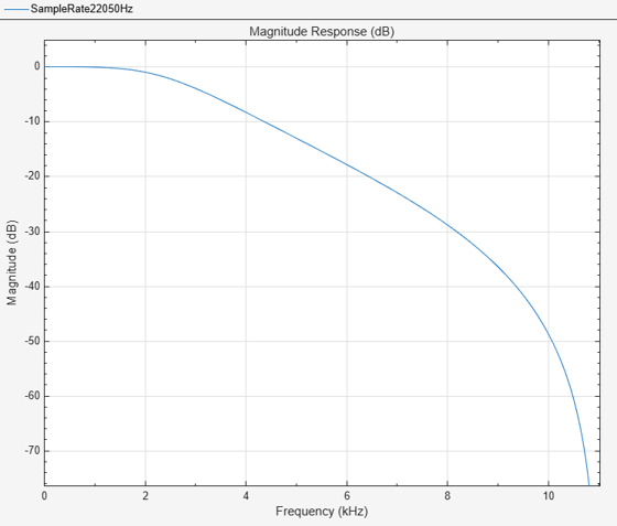
To specify the input sample rate after constructing the object, use the setInputSampleRate function.
setInputSampleRate(sosFilt,44100)
To confirm, view the sample rate information using the info function.
info(sosFilt)
ans = 7×70 char array
    'Discrete-Time IIR Filter (real)                                       '
    '-------------------------------                                       '
    'Filter Structure    : Direct-Form II Transposed, Second-Order Sections'
    'Number of Sections  : 1                                               '
    'Stable              : Yes                                             '
    'Linear Phase        : No                                              '
    'Input sample rate : 44100                                             '
Visualize the frequency response of the filter using filterAnalyzer. Note the change in frequency interval from 0 to 22050 Hz.
filterAnalyzer(sosFilt,FilterNames="SampleRate44100Hz")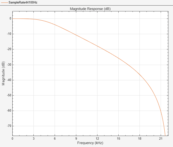
Design a lowpass IIR filter of order 8 using the designLowpassIIR function. Set the SystemObject flag to true to generate a dsp.SOSFilter object. Set HasScaleValues to true.
sosFilt = designLowpassIIR(FilterOrder=8,HasScaleValues=true,...
    SystemObject=true)
sosFilt =
dsp.SOSFilter with properties:
Structure: 'Direct form II transposed'
CoefficientSource: 'Property'
Numerator: [4×3 double]
Denominator: [4×3 double]
HasScaleValues: true
ScaleValues: [0.1287 0.1051 0.0922 0.0865 1]
Show all properties
Use the ctf function to obtain the filter coefficients in the CTF format. The function also outputs the scale values.
[sosnum,sosden,sv] = ctf(sosFilt)
sosnum = 4×3

     1     2     1
     1     2     1
     1     2     1
     1     2     1
sosden = 4×3

    1.0000   -1.2428    0.7575
    1.0000   -1.0153    0.4359
    1.0000   -0.8906    0.2595
    1.0000   -0.8351    0.1810
sv = 5×1

    0.1287
    0.1051
    0.0922
    0.0865
    1.0000
More About
These diagrams show the filter structures supported by the second-order section filter.
This is the structure of each section in the filter when you set the filter structure to
Direct form I.

This is the structure of the filter with P sections when you specify scale values [g1, g2, …, gP+1].

This is the structure of the filter when you do not specify scale values.

This is the structure of each section in the filter when you set the filter structure to
Direct form I transposed.

This is the structure of the filter with P sections when you specify scale values [g1, g2, …, gP+1].
This is the structure of the filter when you do not specify scale values.
This is the structure of each section in the filter when you set the filter structure to
Direct form II.

This is the structure of the filter with P sections when you specify scale values [g1, g2, …, gP+1].
This is the structure of the filter when you do not specify scale values.
This is the structure of each section in the filter when you set the filter structure to
Direct form II transposed.

This is the structure of the filter with P sections when you specify scale values [g1, g2, …, gP+1].
This is the structure of the filter when you do not specify scale values.
These diagrams show the data types used in the SOS filter when the input is fixed-point. For each structure the filter supports, the data types shown in the diagrams can be set through the respective fixed-point settings.
Here is the structure of each section when you set the filter structure to Direct form I. This diagram shows the data types when you input fixed-point signals. The gain operations b0, b1, b2, a1, and a2 operate in full precision.

These diagrams show the fixed-point data types between filter sections.
When the data is not optimized:

When you specify scale values to 1:

Here is the structure of each section when you set the filter structure to Direct form I transposed. This diagram shows the data types when you input fixed-point signals. The dashed casts are omitted when you set HasScaleValues to false. The gain operations b0, b1, b2, a1, and a2 operate in full precision.

These diagrams show the fixed-point data types between filter sections.
When the data is not optimized:

When you specify scale values to 1:

Here is the structure of each section when you set the filter structure to Direct form II. This diagram shows the data types when you input fixed-point signals. The dashed casts are omitted when you set HasScaleValues to false. The gain operations b0, b1, b2, a1, and a2 operate in full precision.

These diagrams show the fixed-point data types between filter sections.
When the data is not optimized:

When you set scale values to 1:

Here is the structure of each section when you set the filter structure to Direct form II transposed. This diagram shows the data types when you input fixed-point signals. The gain operations b0, b1, b2, a1, and a2 operate in full precision. When you set HasScaleValues to false, the data type at the section output is automatically determined by the object algorithm and is not controlled by the value of the SectionOutputDataType property.

These diagrams show the fixed-point data types between filter sections.
When the data is not optimized:

When you specify scale values to 1:

Extended Capabilities
Version History
Introduced in R2020aSee Also
Functions
freqz|filterAnalyzer|impz|info|coeffs|cost|scale|scaleopts|scalecheck|cumsec|tf|scaleFilterSections|outputDelay|setInputSampleRate|designLowpassIIR|designHighpassIIR|designBandpassIIR|designBandstopIIR|designNotchPeakIIR