dsp.FIRInterpolator
Perform polyphase FIR interpolation
Description
The dsp.FIRInterpolator
System object™ performs an efficient polyphase interpolation using an integer upsampling factor
L along the first dimension.
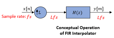
Conceptually, the FIR interpolator (as shown in the schematic) consists of an upsampler
followed by an FIR anti-imaging filter, which is usually an approximation of an ideal
band-limited interpolation filter. The coefficients of the anti-imaging filter can be
specified through the Numerator property, or can be automatically
designed by the object using the designMultirateFIR function.
The upsampler upsamples each channel of the input to a higher rate by inserting L–1 zeros between samples. The FIR filter that follows filters each channel of the upsampled data. The resulting discrete-time signal has a sample rate that is L times the original sample rate.
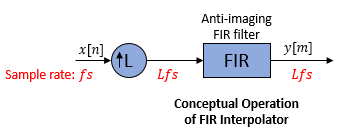
Note that the actual object algorithm implements a direct-form FIR polyphase structure, an efficient equivalent of the combined system depicted in the diagram. For more details, see Algorithms.
To upsample an input:
Create the
dsp.FIRInterpolatorobject and set its properties.Call the object with arguments, as if it were a function.
To learn more about how System objects work, see What Are System Objects?
This object supports C/C++ code generation and SIMD code generation under certain conditions. For more information, see Code Generation.
Creation
Syntax
Description
firinterp = dsp.FIRInterpolatordesignMultirateFIR(3,1) function.
firinterp = dsp.FIRInterpolator(L)InterpolationFactor property set to
L. The object designs its filter coefficients
based on the interpolation factor L that you
specify while creating the object using the
designMultirateFIR(L=1) function. The designed
filter corresponds to a lowpass with a cutoff at
π/L in radial frequency units.
firinterp = dsp.FIRInterpolator(L,"Auto")NumeratorSource property set to
"Auto". In this mode, every time there is an
update in the interpolation factor, the object redesigns the filter
using the design method specified in
DesignMethod.
firinterp = dsp.FIRInterpolator(L,num)InterpolationFactor property set to
L and the Numerator
property set to num.
firinterp = dsp.FIRInterpolator(L,method)InterpolationFactor property set to
L and the DesignMethod
property set to method. When you pass the design
method as an input, the NumeratorSource property
is automatically set to "Auto".
firinterp = dsp.FIRInterpolator(___,InputSampleRate=Value)"normalized". (since R2026a)
To specify an input sample rate of 22050 Hz, set
InputSampleRate to 22050. To specify the input sample rate in
normalized units, set InputSampleRate to
"normalized". (since R2026a)
firinterp = dsp.FIRInterpolator(___,PropertyName=Value)InterpolationFactor to 6.
firinterp = dsp.FIRInterpolator(L,"legacy")fir1(15,0.25). The designed filter has a
cutoff frequency of 0.25π radians/sample.
Properties
Usage
Description
Input Arguments
Output Arguments
Object Functions
To use an object function, specify the
System object as the first input argument. For
example, to release system resources of a System object named obj, use
this syntax:
release(obj)
Examples
Interpolate a cosine wave by a factor of 2. In the automatic filter design mode, change the underlying D/A signal interpolation model to "linear" and interpolate the signal by a factor of 4, change the underlying D/A signal interpolation model to "ZOH" and interpolate the signal by a factor of 5.
The cosine wave has an angular frequency of radians/sample.
x = cos(pi/4*(0:39)');
Design Default Filter
Create a dsp.FIRInterpolator object. The object uses an anti-imaging lowpass filter after upsampling. By default, the anti-imaging lowpass filter is designed using the designMultirateFIR function. The function designs the filter based on the interpolation factor that you specify, and stores the coefficients in the Numerator property. For an interpolation factor of 2, the object designs the coefficients using designMultirateFIR(2,1).
firinterp = dsp.FIRInterpolator(2)
firinterp =
  dsp.FIRInterpolator with properties:

    InterpolationFactor: 2
        NumeratorSource: 'Property'
              Numerator: [0 -2.0108e-04 0 7.7408e-04 0 -0.0020 0 0.0045 0 -0.0086 0 0.0153 0 -0.0257 0 0.0415 0 -0.0661 0 0.1084 0 -0.2003 0 0.6326 1 0.6326 0 -0.2003 0 0.1084 0 -0.0661 0 0.0415 0 -0.0257 0 0.0153 0 -0.0086 0 0.0045 0 … ] (1×48 double)

  Show all properties
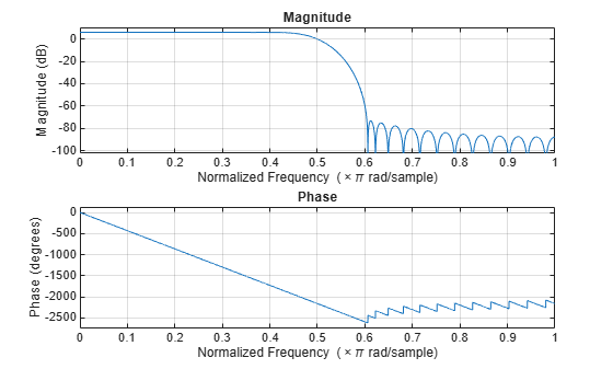
Visualize the filter response. The designed filter meets the ideal filter constraints that are marked in red. The cutoff frequency is approximately half the spectrum.
freqz(firinterp)
Interpolate by 2
Interpolate the cosine signal by a factor of 2.
y = firinterp(x);
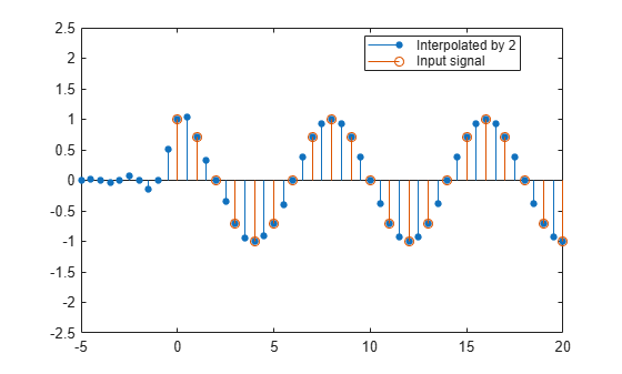
Plot the original and interpolated signals. In order to plot the two signals on the same plot, you must account for the output delay of the FIR interpolator and the scaling introduced by the filter. Use the outputDelay function to compute the delay value introduced by the interpolator. Shift the output by this delay value.
Visualize the input and the resampled signals. The input and output values coincide every other sample, due to the interpolation factor of 2.
[delay,FsOut] = outputDelay(firinterp)
delay =
12
FsOut =
2
nx = (0:length(x)-1);
ty = (0:length(y)-1)/FsOut-delay;
stem(ty,y,"filled",MarkerSize=4); hold on;
stem(nx,x); hold off;
xlim([-5,20])
ylim([-2.5 2.5])
legend("Interpolated by 2","Input signal","Location","best");
Interpolate by 4 in Automatic Filter Design Mode
Now interpolate by a factor of 4. In order for the filter design to be updated automatically based on the new interpolation factor, set the NumeratorSource property to "Auto". Alternately, you can pass the keyword "Auto" as an input while creating the object. The object then operates in the automatic filter design mode. Every time there is a change in the interpolation factor, the object updates the filter design.
release(firinterp)
firinterp.NumeratorSource = "Auto";
firinterp.InterpolationFactor = 4
firinterp =
dsp.FIRInterpolator with properties:
InterpolationFactor: 4
NumeratorSource: 'Auto'
DesignMethod: 'Kaiser'
Show all properties
To access the filter coefficients in the automatic filter design mode, type firinterp.Numerator in the MATLAB command prompt.
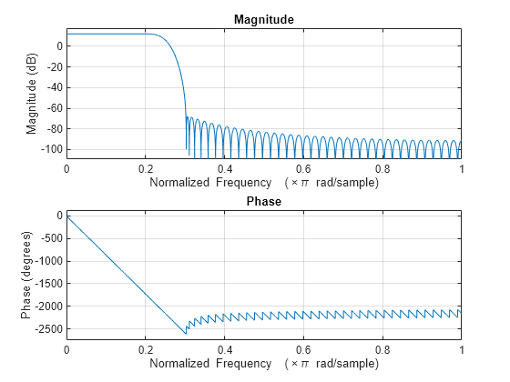
The designed filter occupies a narrower passband that is approximately a quarter of the spectrum.
freqz(firinterp)
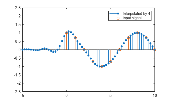
Interpolate the cosine signal by a factor of 4.
yAuto = firinterp(x);
Plot the original and resampled signals. Recalculate the delay and the output sample rate values since the interpolation factor has changed. The input and output values coincide every 4 output samples, owing to the interpolation factor of 4.
[delay,FsOut] = outputDelay(firinterp);

nx = (0:length(x)-1);
tyAuto = (0:length(yAuto)-1)/FsOut-delay;
stem(tyAuto,yAuto,"filled",MarkerSize=4); hold on;
stem(nx,x); hold off;
xlim([-5,10])
ylim([-2.5 2.5])
legend("Interpolated by 4","Input signal");
Specify Signal Interpolation Model
In the automatic design mode, you can also specify the underlying D/A signal interpolation model through the DesignMethod property.
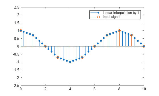
Set DesignMethod to "linear"
If you set the DesignMethod to "linear", the object uses the linear interpolation model.
release(firinterp)
firinterp.DesignMethod = "linear"
firinterp =
dsp.FIRInterpolator with properties:
InterpolationFactor: 4
NumeratorSource: 'Auto'
DesignMethod: 'Linear'
Show all properties
Interpolate the signal using the linear interpolation model.
ylinear = firinterp(x);
Plot the original and the linearly interpolated signal.
[delay,FsOut] = outputDelay(firinterp);
nx = (0:length(x)-1);

% Calculate output times for vector ylinear in input units
tylinear = (0:length(ylinear)-1)/FsOut-delay;

stem(tylinear,ylinear,"filled",MarkerSize=4); hold on;
stem(nx,x);
hold off;
xlim([0,10])
ylim([-2.5 2.5])
legend("Linear Interpolation by 4","Input signal");
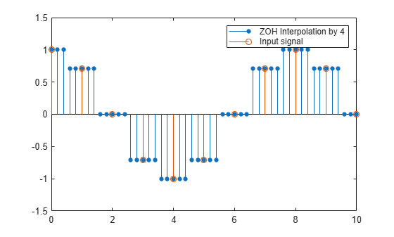
Set DesignMethod to "ZOH" and Change InterpolationFactor to 5
If you set the DesignMethod to "ZOH", the object uses the zero order hold method. Change the interpolation factor to 5.
release(firinterp)
firinterp.DesignMethod = "ZOH";
firinterp.InterpolationFactor = 5
firinterp =
dsp.FIRInterpolator with properties:
InterpolationFactor: 5
NumeratorSource: 'Auto'
DesignMethod: 'ZOH'
Show all properties
Interpolate the signal using the zero order hold method.
yzoh = firinterp(x);
Plot the original and ZOH interpolated signal.
[delay,FsOut] = outputDelay(firinterp);
nx = (0:length(x)-1);

% Calculate output times for vector yzoh in input units
tyzoh = (0:length(yzoh)-1)/FsOut-delay;

stem(tyzoh,yzoh,"filled",MarkerSize=4); hold on;
stem(nx,x); hold off;
xlim([0,10])
ylim([-1.5 1.5])
legend("ZOH Interpolation by 4","Input signal");
Double the sample rate of an audio signal and play the interpolated signal using the audioDeviceWriter object.
Note: The audioDeviceWriter System object™ is not supported in MATLAB Online.
Create a dsp.AudioFileReader object. The default audio file ready by the object has a sample rate of 22050 Hz.
afr = dsp.AudioFileReader(OutputDataType="single");Create a dsp.FIRInterpolator object and specify the interpolation factor to be 2. The object designs the filter using the designMultirateFIR(2,1) function and stores the coefficients in the Numerator property of the object.
firInterp = dsp.FIRInterpolator(2)
firInterp =
  dsp.FIRInterpolator with properties:

    InterpolationFactor: 2
        NumeratorSource: 'Property'
              Numerator: [0 -2.0108e-04 0 7.7408e-04 0 -0.0020 0 0.0045 0 -0.0086 0 0.0153 0 -0.0257 0 0.0415 0 -0.0661 0 0.1084 0 -0.2003 0 0.6326 1 0.6326 0 -0.2003 0 0.1084 0 -0.0661 0 0.0415 0 -0.0257 0 0.0153 0 -0.0086 0 0.0045 0 … ] (1×48 double)

  Show all properties
Create an audioDeviceWriter object. Specify the sample rate to be 220502, which equals 44100 Hz.
adw = audioDeviceWriter(44100)
adw =
  audioDeviceWriter with properties:

        Device: 'Default'
    SampleRate: 44100

  Show all properties
Read the audio signal using the file reader object, double the sample rate of the signal from 22050 Hz to 44100 Hz and play the interpolated signal.
while ~isDone(afr)
     frame = afr();
     y = firInterp(frame);
     adw(y);
end

pause(1);
release(afr);
release(adw);
Since R2026a
Specify the input sample rate explicitly while constructing the dsp.FIRInterpolator object using the InputSampleRate argument.
firInterp = dsp.FIRInterpolator(InputSampleRate=22050)
firInterp =
  dsp.FIRInterpolator with properties:

    InterpolationFactor: 3
        NumeratorSource: 'Property'
              Numerator: [0 -1.2906e-04 -2.2804e-04 0 5.5461e-04 8.0261e-04 0 -0.0015 -0.0020 0 0.0034 0.0043 0 -0.0067 -0.0083 0 0.0121 0.0145 0 -0.0205 -0.0241 0 0.0332 0.0388 0 -0.0530 -0.0620 0 0.0861 0.1027 0 -0.1540 -0.1976 0 … ] (1×72 double)

  Show all properties
You can view this information using the Input sample rate field of the info function.
info(firInterp)
ans = 11×62 char array
    'Discrete-Time FIR Multirate Filter (real)                     '
    '-----------------------------------------                     '
    'Filter Structure      : Direct-Form FIR Polyphase Interpolator'
    'Interpolation Factor  : 3                                     '
    'Polyphase Length      : 24                                    '
    'Filter Length         : 72                                    '
    'Stable                : Yes                                   '
    'Linear Phase          : Yes (Type 1)                          '
    '                                                              '
    'Arithmetic            : double                                '
    'Input sample rate : 22050                                     '
Visualize the frequency response of the filter using filterAnalyzer. Note the frequency range from 0 to 11025 Hz.
filterAnalyzer(firInterp,FilterNames="InputSampleRate22050Hz")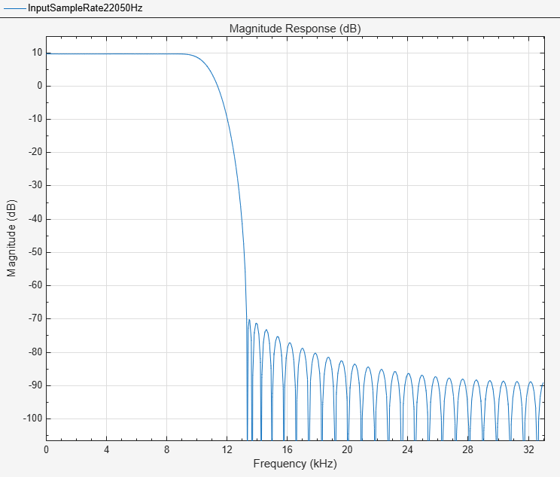
To specify the input sample rate after constructing the object, use the setInputSampleRate function.
setInputSampleRate(firInterp,44100)
To confirm, view the sample rate information using the info function.
info(firInterp)
ans = 11×62 char array
    'Discrete-Time FIR Multirate Filter (real)                     '
    '-----------------------------------------                     '
    'Filter Structure      : Direct-Form FIR Polyphase Interpolator'
    'Interpolation Factor  : 3                                     '
    'Polyphase Length      : 24                                    '
    'Filter Length         : 72                                    '
    'Stable                : Yes                                   '
    'Linear Phase          : Yes (Type 1)                          '
    '                                                              '
    'Arithmetic            : double                                '
    'Input sample rate : 44100                                     '
Visualize the frequency response of the filter using filterAnalyzer. Note the change in frequency interval from 0 to 22050 Hz.
filterAnalyzer(firInterp,FilterNames="InputSampleRate44100Hz")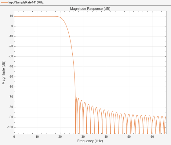
Algorithms
The FIR interpolation filter is implemented efficiently using a polyphase structure.
To derive the polyphase structure, start with the transfer function of the FIR filter:
N+1 is the length of the FIR filter.
You can rearrange this equation as follows:
L is the number of polyphase components, and its value equals the interpolation factor that you specify.
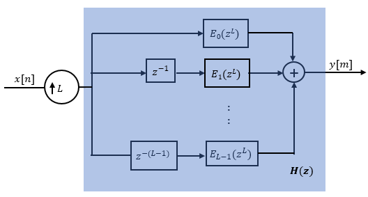
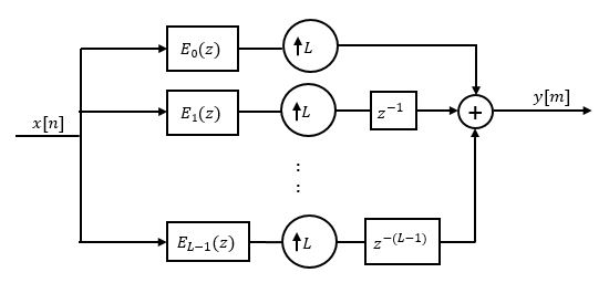
You can write this equation as:
E0(zL), E1(zL), ..., EL-1(zL) are polyphase components of the FIR filter H(z).
Conceptually, the FIR interpolation filter contains an upsampler followed by an FIR lowpass filter H(z).
Replace H(z) with its polyphase representation.
Here is the multirate noble identity for interpolation.
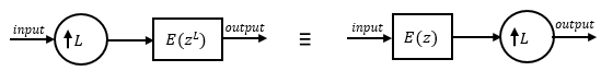
Applying the noble identity for interpolation moves the upsampling operation to after the filtering operation. This move enables you to filter the signal at a lower rate.
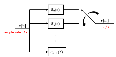
You can replace the upsampling operator, delay block, and adder with a commutator switch. The switch starts on the first branch 0 and moves in the counterclockwise direction, each time receiving one sample from each branch. The interpolator effectively outputs L samples for every one input sample it receives. Hence the sample rate at the output of the FIR interpolation filter is Lfs.
Extended Capabilities
Version History
Introduced in R2012aSee Also
Functions
freqz|freqzmr|filterAnalyzer|info|cost|polyphase|impz|coeffs|outputDelay|designRateConverter|setInputSampleRate