PolarAxes Properties

Polar axes appearance and behavior

PolarAxes properties control the appearance and behavior of a PolarAxes object. By changing property values, you can modify certain aspects of the polar axes. Set axes properties after plotting since some graphics functions reset axes properties.

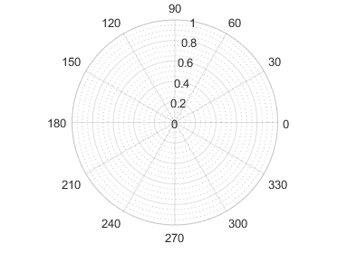
Some graphics functions create polar axes when plotting. Use gca to access the newly created axes. To create empty polar axes, use the polaraxes function.

polarplot([0 pi/2 pi],[1 2 3])
ax = gca;
d = ax.ThetaDir;
ax.ThetaDir = 'clockwise';

Font

FontName — Font name

supported font name | "FixedWidth"

Font name, specified as a supported font name or "FixedWidth". To display and print text properly, you must choose a font that your system supports. The default font depends on your operating system and locale.

To use a fixed-width font that looks good in any locale, use "FixedWidth". The fixed-width font relies on the root FixedWidthFontName property. Setting the root FixedWidthFontName property causes an immediate update of the display to use the new font.

FontSize — Font size

scalar numeric value

Font size, specified as a scalar numeric value. The font size affects the title and tick labels. It also affects any legends or colorbars associated with the axes. The default font size depends on the specific operating system and locale. By default, the font size is measured in points. To change the units, set the FontUnits property.

MATLAB^® automatically scales some of the text to a percentage of the axes font size.

• Titles — 110% of the axes font size by default. To control the scaling, use the TitleFontSizeMultiplier and LabelFontSizeMultiplier properties.

• Legends and colorbars — 90% of the axes font size by default. To specify a different font size, set the FontSize property for the Legend or Colorbar object instead.

Example: ax.FontSize = 12

FontSizeMode — Selection mode for font size

'auto' (default) | 'manual'

Selection mode for the font size, specified as one of these values:

• 'auto' — Font size specified by MATLAB. If you resize the axes to be smaller than the default size, the font size might scale down to improve readability and layout.

• 'manual' — Font size specified manually. Do not scale the font size as the axes size changes. To specify the font size, set the FontSize property.

FontWeight — Character thickness

'normal' (default) | 'bold'

Character thickness, specified as 'normal' or 'bold'.

MATLAB uses the FontWeight property to select a font from those available on your system. Not all fonts have a bold weight. Therefore, specifying a bold font weight can still result in the normal font weight.

FontAngle — Character slant

'normal' (default) | 'italic'

Character slant, specified as 'normal' or 'italic'.

Not all fonts have both font styles. Therefore, the italic font might look the same as the normal font.

TitleFontSizeMultiplier — Scale factor for title font size

1.1 (default) | numeric value greater than 0

Scale factor for the title font size, specified as a numeric value greater than 0. The scale factor is applied to the value of the FontSize property to determine the font size for the title.

TitleFontWeight — Title character thickness

'bold' (default) | 'normal'

Title character thickness, specified as one of these values:

• 'normal' — Default weight as defined by the particular font

• 'bold' — Thicker characters than normal

SubtitleFontWeight — Subtitle character thickness

'normal' (default) | 'bold'

Subtitle character thickness, specified as one of these values:

• 'normal' — Default weight as defined by the particular font

• 'bold' — Thicker characters than normal

FontUnits — Font size units

'points' (default) | 'inches' | 'centimeters' | 'normalized' | 'pixels'

Font size units, specified as one of these values.

Units	Description
'points'	Points. One point equals 1/72 inch.
'inches'	Inches.
'centimeters'	Centimeters.
'normalized'	Interpret font size as a fraction of the axes height. If you resize the axes, the font size modifies accordingly. For example, if the FontSize is 0.1 in normalized units, then the text is 1/10 of the height value stored in the axes Position property.
'pixels'	Pixels. On Windows® and Macintosh systems, the size of a pixel is 1/96th of an inch. This size is independent of your system resolution. On Linux® systems, the size of a pixel is determined by your system resolution.

To set both the font size and the font units in a single function call, you first must set the FontUnits property so that the Axes object correctly interprets the specified font size.

Ticks

RTick — Radius tick values

[0 0.2 0.4 0.6 0.8 1] (default) | vector of increasing values

Radius tick values, specified as a vector of increasing values. The radius tick values are the locations along the r-axis where the circular lines appear. The radius tick labels are the labels that you see next to each line. Use the RTickLabels property to specify the associated labels.

Example: ax.RTick = [0 2 4 6];

Alternatively, use the rticks function to specify the tick values.

RTickMode — Selection mode for radius tick values

'auto' (default) | 'manual'

Selection mode for the radius tick values, specified as one of these values:

• 'auto' — Automatically select the tick values based on the range of data for the axis.

• 'manual' — Manually specify the tick values. To specify the values, set the RTick property.

Example: ax.RTickMode = 'auto'

RTickLabel — Radius tick labels

{'0'; '0.2'; '0.4'; '0.6'; '0.8'; '1'} (default) | cell array of character vectors | string array | categorical array

Radius tick labels, specified as a cell array of character vectors, string array, or categorical array. If you do not want tick labels to show, then specify an empty cell array {}. If you do not specify enough labels for all the ticks values, then the labels repeat.

Tick labels support TeX and LaTeX markup. See the TickLabelInterpreter property for more information.

If you specify this property as a categorical array, MATLAB uses the values in the array, not the categories.

Example: ax.RTickLabel = {'one','two','three','four'};

Alternatively, use the rticklabels function.

RTickLabelMode — Selection mode for RTickLabel

'auto' (default) | 'manual'

Selection mode for the RTickLabel property value, specified as one of these values:

• 'auto' — Automatically select the tick labels.

• 'manual' — Manually specify the tick labels. To specify the labels, set the RTickLabel property.

ThetaTick — Angles at which to display lines

[0 30 60 ... 300 330 360] (default) | vector of increasing values

Angles at which to display lines extending from the origin, specified as a vector of increasing values. MATLAB labels the lines with the appropriate angle values, unless you specify different labels using the ThetaTickLabel property.

MATLAB interprets the values in units determined by the ThetaAxisUnits property.

Example: ax.ThetaTick = [0 90 180 270];

Alternatively, specify the values using the thetaticks function.

ThetaTickMode — Selection mode for ThetaTick

'auto' (default) | 'manual'

Selection mode for the ThetaTick property value, specified as one of these values:

• 'auto' — Automatically select the property value.

• 'manual' — Use the specified property value. To specify the value, set the ThetaTick property.

ThetaTickLabel — Labels for angle lines

{'0'; '30'; '60'; ... '300'; '330'; '360'} (default) | cell array of character vectors | string array | categorical array

Labels for angle lines, specified as a cell array of character vectors, string array, or categorical array.

If you do not specify enough labels for all the lines, then the labels repeat. Labels support TeX and LaTeX markup. See the TickLabelInterpreter property for more information.

If you specify this property as a categorical array, MATLAB uses the values in the array, not the categories.

Example: ax.ThetaTickLabel = {'right','top','left','bottom'};

Alternatively, specify the values using the thetaticklabels function.

ThetaTickLabelMode — Selection mode for ThetaTickLabel

'auto' (default) | 'manual'

Selection mode for the ThetaTickLabel property value, specified as one of these values:

• 'auto' — Automatically select the property value.

• 'manual' — Use the specified property value. To specify the value, set the ThetaTickLabel property.

RTickLabelRotation — Rotation of r-axis tick labels

0 (default) | scalar value in degrees

Rotation of r-axis tick labels, specified as a scalar value in degrees. Positive values give counterclockwise rotation. Negative values give clockwise rotation.

Example: ax.RTickLabelRotation = 45;

Alternatively, use the rtickangle function.

RTickLabelRotationMode — Selection mode for tick label rotation

'auto' (default) | 'manual'

Selection mode for the r-axis tick label rotation, specified as one of these values:

• 'auto' — Automatically select the tick label rotation.

• 'manual' — Use a tick label rotation that you specify. To specify the rotation, set the RTickLabelRotation property.

RMinorTick — Minor tick marks along r-axis

'off' | on/off logical value

Minor tick marks along r-axis, specified as 'on' or 'off', or as numeric or logical 1 (true) or 0 (false). A value of 'on' is equivalent to true, and 'off' is equivalent to false. Thus, you can use the value of this property as a logical value. The value is stored as an on/off logical value of type matlab.lang.OnOffSwitchState.

• 'on' — Display minor tick marks. The space between the major tick marks and grid lines determines the number of minor tick marks. This property value has a visual effect only if the tick length is positive (controlled by the TickLength property) and if the polar axes is a full circle (controlled by the ThetaLim property).

• 'off' — Do not display minor tick marks.

Example: ax.RMinorTick = 'on';

ThetaMinorTick — Minor tick marks between angle lines

'off' (default) | on/off logical value

Minor tick marks between angle lines, specified as 'on' or 'off', or as numeric or logical 1 (true) or 0 (false). A value of 'on' is equivalent to true, and 'off' is equivalent to false. Thus, you can use the value of this property as a logical value. The value is stored as an on/off logical value of type matlab.lang.OnOffSwitchState.

• 'on' — Display minor tick marks. The space between the lines determines the number of minor tick marks. This property value has a visual effect only if the tick length is positive. To set the tick length, use the TickLength property, for example, ax.TickLength = [0.02 0].

• 'off' — Do not display minor tick marks.

ThetaZeroLocation — Location of the zero reference axis

"right" (default) | "top" | "left" | "bottom" | angle value (since R2025a)

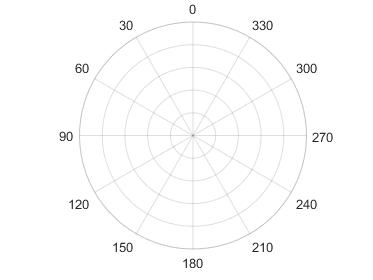
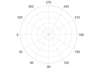
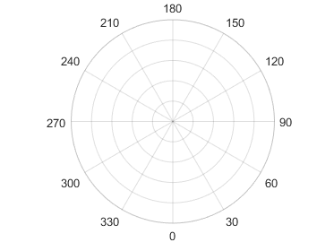
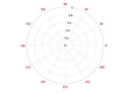
Location of the zero reference axis, specified as "right", "top", "left", "bottom", or an angle value. If you specify an angle value, be sure to a specify the value in degrees or radians, according to the ThetaAxisUnits property. By default, the ThetaAxisUnits property is set to "degrees".

Value	Result
"right"
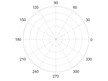
"top"
"left"
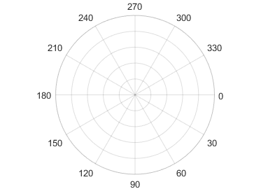
"bottom"
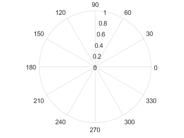
45

Example: polaraxes(ThetaZeroLocation="left")

Example: polaraxes(ThetaZeroLocation=45)

TickDir — Tick mark direction

'in' (default) | 'out' | 'both' | 'none'

Tick mark direction, specified as one of these values:

• 'in' — Direct the tick marks inward from the axis lines. (Default for 2-D views)

• 'out' — Direct the tick marks outward from the axis lines. (Default for 3-D views)

• 'both' — Center the tick marks over the axis lines.

• 'none' — Do not display any tick marks.

TickDirMode — Selection mode for TickDir

'auto' (default) | 'manual'

Selection mode for the TickDir property, specified as one of these values:

• 'auto' — Automatically select the tick direction based on the current view.

• 'manual' — Manually specify the tick direction. To specify the tick direction, set the TickDir property.

Example: ax.TickDirMode = 'auto'

TickLabelInterpreter — Tick label interpreter

'tex' (default) | 'latex' | 'none'

Tick label interpreter, specified as one of these values:

• 'tex' — Interpret labels using a subset of the TeX markup.

• 'latex' — Interpret labels using a subset of LaTeX markup. When you specify the tick labels, use dollar signs around each element in the cell array.

• 'none' — Display literal characters.

TeX Markup

By default, MATLAB supports a subset of TeX markup. Use TeX markup to add superscripts and subscripts, modify the text type and color, and include special characters in the labels.

Modifiers remain in effect until the end of the text. Superscripts and subscripts are an exception because they modify only the next character or the characters within the curly braces. When you set the interpreter to "tex", the supported modifiers are as follows.

Modifier	Description	Example
^{ }	Superscript	"text^{superscript}"
_{ }	Subscript	"text_{subscript}"
\bf	Bold font	"\bf text"
\it	Italic font	"\it text"
\sl	Oblique font (usually the same as italic font)	"\sl text"
\rm	Normal font	"\rm text"
\fontname{specifier}	Font name — Replace specifier with the name of a font family. You can use this in combination with other modifiers.	"\fontname{Courier} text"
\fontsize{specifier}	Font size —Replace specifier with a numeric scalar value in point units.	"\fontsize{15} text"
\color{specifier}	Font color — Replace specifier with one of these colors: red, green, yellow, magenta, blue, black, white, gray, darkGreen, orange, or lightBlue.	"\color{magenta} text"
\color[rgb]{specifier}	Custom font color — Replace specifier with a three-element RGB triplet.	"\color[rgb]{0,0.5,0.5} text"

This table lists the supported special characters for the "tex" interpreter.

Character Sequence	Symbol	Character Sequence	Symbol	Character Sequence	Symbol
\alpha	α	\upsilon	υ	\sim	~
\angle	∠	\phi	ϕ	\leq	≤
\ast	*	\chi	χ	\infty	∞
\beta	β	\psi	ψ	\clubsuit	♣
\gamma	γ	\omega	ω	\diamondsuit	♦
\delta	δ	\Gamma	Γ	\heartsuit	♥
\epsilon	ϵ	\Delta	Δ	\spadesuit	♠
\zeta	ζ	\Theta	Θ	\leftrightarrow	↔
\eta	η	\Lambda	Λ	\leftarrow	←
\theta	θ	\Xi	Ξ	\Leftarrow	⇐
\vartheta	ϑ	\Pi	Π	\uparrow	↑
\iota	ι	\Sigma	Σ	\rightarrow	→
\kappa	κ	\Upsilon	ϒ	\Rightarrow	⇒
\lambda	λ	\Phi	Φ	\downarrow	↓
\mu	µ	\Psi	Ψ	\circ	º
\nu	ν	\Omega	Ω	\pm	±
\xi	ξ	\forall	∀	\geq	≥
\pi	π	\exists	∃	\propto	∝
\rho	ρ	\ni	∍	\partial	∂
\sigma	σ	\cong	≅	\bullet	•
\varsigma	ς	\approx	≈	\div	÷
\tau	τ	\Re	ℜ	\neq	≠
\equiv	≡	\oplus	⊕	\aleph	ℵ
\Im	ℑ	\cup	∪	\wp	℘
\otimes	⊗	\subseteq	⊆	\oslash	∅
\cap	∩	\in	∈	\supseteq	⊇
\supset	⊃	\lceil	⌈	\subset	⊂
\int	∫	\cdot	·	\o	ο
\rfloor	⌋	\neg	¬	\nabla	∇
\lfloor	⌊	\times	x	\ldots	...
\perp	⊥	\surd	√	\prime	´
\wedge	∧	\varpi	ϖ	\0	∅
\rceil	⌉	\rangle	〉	\mid	|
\vee	∨	\langle	〈	\copyright	©

LaTeX Markup

To use LaTeX markup, set the TickLabelInterpreter property to 'latex'. Use dollar symbols around the labels, for example, use '$\int_1^{20} x^2 dx$' for inline mode or '$$\int_1^{20} x^2 dx$$' for display mode.

The displayed text uses the default LaTeX font style. The FontName, FontWeight, and FontAngle properties do not have an effect. To change the font style, use LaTeX markup within the text. The maximum size of the text that you can use with the LaTeX interpreter is 1200 characters. For multiline text, the maximum size of the text reduces by about 10 characters per line.

MATLAB supports most standard LaTeX math mode commands. For more information, see Supported LaTeX Commands. For examples that use TeX and LaTeX, see Greek Letters and Special Characters in Chart Text.

TickLength — Tick mark length

[0 0] (default) | two-element vector

Tick mark length, specified as a two-element vector. The first element determines the tick length. The second element is ignored.

Example: ax.TickLength = [0.02 0];

Rulers

RLim — Minimum and maximum radius limits

[0 1] (default) | two-element vector of the form [rmin rmax]

Minimum and maximum radius limits, specified as a two-element vector of the form [rmin rmax], where rmax is a numeric value greater than rmin. You can specify both limits, or specify one limit and let the axes automatically calculate the other.

• To automatically set the minimum limit to the minimum data value, specify the first element as -inf, for example, [-inf 0].

• To automatically set the maximum limit to the maximum data value, specify the second element as inf, for example, [0 inf].

Alternatively, use the rlim function to set the limits.

Example: ax.RLim = [0 6];

RLimMode — Selection mode for RLim

'auto' (default) | 'manual

Selection mode for the RLim property value, specified as one of these values:

• 'auto'— Automatically set the property value.

• 'manual'— Use the specified property value. To specify the value, set the RLim property.

ThetaLim — Minimum and maximum angle values

[0 360] (default) | two-element vector of the form [thmin thmax]

Minimum and maximum angle values, specified as a two-element vector of the form [thmin thmax]. If the difference between the values is less than 360 degrees, then the theta-axis is a partial circle.

MATLAB interprets the values in units determined by the ThetaAxisUnits property.

Example: ax.ThetaLim = [0 180];

ThetaLimMode — Selection mode for ThetaLim

'auto' (default) | 'manual

Selection mode for the ThetaLim property value, specified as one of these values:

• 'auto' — Automatically select the property value.

• 'manual' — Use the specified property value. To specify the value, set the ThetaLim property.

RAxis — Component that controls appearance and behavior of r-axis

ruler object (default)

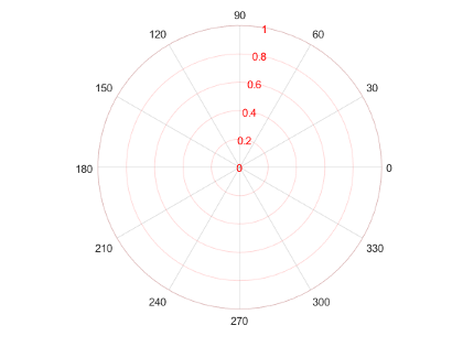
Component that controls the appearance and behavior of the r-axis, returned as a ruler object. When MATLAB creates polar axes, it automatically creates a ruler for the r-axis. Modify the appearance and behavior of this axis by accessing the associated ruler and setting ruler properties. For a list of options, see NumericRuler Properties.

For example, change the color of the r-axis to red.

ax = polaraxes;
ax.RAxis.Color = 'r';

Use the RAxis properties to access the ruler objects and set ruler properties. If you want to set polar axes properties, set them directly on the PolarAxes object.

ThetaAxis — Component that controls appearance and behavior of theta-axis

ruler object (default)

Component that controls the appearance and behavior of the theta-axis, returned as a ruler object. When MATLAB creates polar axes, it automatically creates a numeric ruler for the theta-axis. Modify the appearance and behavior of this axis by accessing the associated ruler and setting ruler properties. For a list of options, see NumericRuler Properties.

For example, change the color of the theta-axis to red.

ax = polaraxes;
ax.ThetaAxis.Color = 'r';

Use the ThetaAxis property to access the ruler object and set ruler properties. If you want to set polar axes properties, set them directly on the PolarAxes object.

RAxisLocation — Location of r-axis

80 (default) | scalar angle value

Location of the r-axis, specified a scalar angle value. MATLAB interprets the values in units determined by the ThetaAxisUnits property.

Example: ax.RAxisLocation = 90;

RAxisLocationMode — Selection mode for RAxisLocation

'auto' (default) | 'manual'

Selection mode for the RAxisLocation property value, specified as one of these values:

• 'auto' — Automatically select the property value.

• 'manual' — Use the specified property value. To specify the value, set the RAxisLocation property.

RColor — Color of r-axis

RGB triplet | hexadecimal color code | 'r' | 'g' | 'b' | ...

Color of the r-axis, including the r-axis grid lines, tick marks, and tick labels. Specify this value as an RGB triplet, a hexadecimal color code, a color name, or a short name.

Note

If you specify the GridColor property, then the grid lines use the color in the GridColor property instead. See GridColorMode for more information.

For a custom color, specify an RGB triplet or a hexadecimal color code.

• An RGB triplet is a three-element row vector whose elements specify the intensities of the red, green, and blue components of the color. The intensities must be in the range [0,1], for example, [0.4 0.6 0.7].

• A hexadecimal color code is a string scalar or character vector that starts with a hash symbol (#) followed by three or six hexadecimal digits, which can range from 0 to F. The values are not case sensitive. Therefore, the color codes "#FF8800", "#ff8800", "#F80", and "#f80" are equivalent.

Alternatively, you can specify some common colors by name. This table lists the named color options, the equivalent RGB triplets, and the hexadecimal color codes.

Color Name	Short Name	RGB Triplet	Hexadecimal Color Code	Appearance
"red"	"r"	[1 0 0]	"#FF0000"
"green"	"g"	[0 1 0]	"#00FF00"
"blue"	"b"	[0 0 1]	"#0000FF"
"cyan"	"c"	[0 1 1]	"#00FFFF"
"magenta"	"m"	[1 0 1]	"#FF00FF"
"yellow"	"y"	[1 1 0]	"#FFFF00"
"black"	"k"	[0 0 0]	"#000000"
"white"	"w"	[1 1 1]	"#FFFFFF"
"none"	Not applicable	Not applicable	Not applicable	No color

This table lists the default color palettes for plots in the light and dark themes.

Palette	Palette Colors
"gem" — Light theme default Before R2025a: Most plots use these colors by default.
"glow" — Dark theme default

You can get the RGB triplets and hexadecimal color codes for these palettes using the orderedcolors and rgb2hex functions. For example, get the RGB triplets for the "gem" palette and convert them to hexadecimal color codes.

RGB = orderedcolors("gem");
H = rgb2hex(RGB);

Before R2023b: Get the RGB triplets using RGB = get(groot,"FactoryAxesColorOrder").

Before R2024a: Get the hexadecimal color codes using H = compose("#%02X%02X%02X",round(RGB*255)).

For example, ax.RColor = 'r' changes the color to red.

RColorMode — Property for setting r-axis grid color

'auto' (default) | 'manual'

Property for setting r-axis grid color, specified 'auto' or 'manual'. The mode value only affects the r-axis grid color. The r-axis tick labels always use the RColor value, regardless of the mode.

The r-axis grid color depends on both the RColorMode property and the GridColorMode property, as shown here.

RColorMode	GridColorMode	r-Axis Grid Color
'auto'	'auto'	GridColor property
	'manual'	GridColor property
'manual'	'auto'	RColor property
	'manual'	GridColor property

The r-axis minor grid color depends on both the RColorMode property and the MinorGridColorMode property, as shown here.

RColorMode	MinorGridColorMode	r-Axis Minor Grid Color
'auto'	'auto'	MinorGridColor property
	'manual'	MinorGridColor property
'manual'	'auto'	RColor property
	'manual'	MinorGridColor property

ThetaColor — Color of theta-axis

RGB triplet | hexadecimal color code | 'r' | 'g' | 'b' | ...

Color of the theta-axis, including the theta-axis grid lines, tick marks, tick labels. Specify this value as an RGB triplet, a hexadecimal color code, a color name, or a short name.

Note

If you specify the GridColor property, then the grid lines use the color in the GridColor property instead. See GridColorMode for more information.

For a custom color, specify an RGB triplet or a hexadecimal color code.

• An RGB triplet is a three-element row vector whose elements specify the intensities of the red, green, and blue components of the color. The intensities must be in the range [0,1], for example, [0.4 0.6 0.7].

• A hexadecimal color code is a string scalar or character vector that starts with a hash symbol (#) followed by three or six hexadecimal digits, which can range from 0 to F. The values are not case sensitive. Therefore, the color codes "#FF8800", "#ff8800", "#F80", and "#f80" are equivalent.

Alternatively, you can specify some common colors by name. This table lists the named color options, the equivalent RGB triplets, and the hexadecimal color codes.

Color Name	Short Name	RGB Triplet	Hexadecimal Color Code	Appearance
"red"	"r"	[1 0 0]	"#FF0000"
"green"	"g"	[0 1 0]	"#00FF00"
"blue"	"b"	[0 0 1]	"#0000FF"
"cyan"	"c"	[0 1 1]	"#00FFFF"
"magenta"	"m"	[1 0 1]	"#FF00FF"
"yellow"	"y"	[1 1 0]	"#FFFF00"
"black"	"k"	[0 0 0]	"#000000"
"white"	"w"	[1 1 1]	"#FFFFFF"
"none"	Not applicable	Not applicable	Not applicable	No color

This table lists the default color palettes for plots in the light and dark themes.

Palette	Palette Colors
"gem" — Light theme default Before R2025a: Most plots use these colors by default.
"glow" — Dark theme default

You can get the RGB triplets and hexadecimal color codes for these palettes using the orderedcolors and rgb2hex functions. For example, get the RGB triplets for the "gem" palette and convert them to hexadecimal color codes.

RGB = orderedcolors("gem");
H = rgb2hex(RGB);

Before R2023b: Get the RGB triplets using RGB = get(groot,"FactoryAxesColorOrder").

Before R2024a: Get the hexadecimal color codes using H = compose("#%02X%02X%02X",round(RGB*255)).

For example, ax.ThetaColor = 'r' changes the color to red.

ThetaColorMode — Property for setting theta-axis grid color

'auto' (default) | 'manual'

Property for setting theta-axis grid color, specified 'auto' or 'manual'. The mode value only affects the theta-axis grid color. The theta-axis line, tick marks, and labels always use the ThetaColor value, regardless of the mode.

The theta-axis grid color depends on both the ThetaColorMode property and the GridColorMode property, as shown here.

ThetaColorMode	GridColorMode	theta-Axis Grid Color
'auto'	'auto'	GridColor property
	'manual'	GridColor property
'manual'	'auto'	ThetaColor property
	'manual'	GridColor property

The theta-axis minor grid color depends on both the ThetaColorMode property and the MinorGridColorMode property, as shown here.

ThetaColorMode	MinorGridColorMode	theta-Axis Minor Grid Color
'auto'	'auto'	MinorGridColor property
	'manual'	MinorGridColor property
'manual'	'auto'	ThetaColor property
	'manual'	MinorGridColor property

RDir — Direction of increasing values along r-axis

'normal' (default) | 'reverse'

Direction of increasing values along the r-axis, specified as one of these values:

• 'normal' — Values increase outward from the center of the chart. The radius at the origin corresponds to the minimum value stored in the RLim property (typically 0).

• 'reverse' — Values decrease outward from the center of the chart. The radius at the origin corresponds to the maximum value stored in the RLim property.

Example: ax.RDir = 'reverse';

ThetaDir — Direction of increasing angles

'counterclockwise' (default) | 'clockwise'

Direction of increasing angles, specified as one of the values in this table.

Value	Result
'counterclockwise'	Angles increase in a counterclockwise direction.
'clockwise'	Angles increase in a clockwise direction.

Example: ax.ThetaDir = 'clockwise';

ThetaAxisUnits — Units for angle values

'degrees' (default) | 'radians'

Units for angle values, specified as one of these values:

• 'degrees' — Label the angles in degrees, and interpret the ThetaLim, ThetaTick, and RAxisLocation property values in degrees. When you switch the units from radians to degrees, MATLAB converts the radian values in those three properties to the equivalent degree values.

• 'radians' — Label the angles in radians, and interpret the ThetaLim, ThetaTick, and RAxisLocation property values in radians. When you switch the units from degrees to radians, MATLAB converts the degree values in those three properties to the equivalent radian values.

Example: ax.ThetaAxisUnits = 'radians';

Grid Lines

RGrid — Display of r-axis grid lines

'on' (default) | on/off logical value

Display of r-axis grid lines, specified as 'on' or 'off', or as numeric or logical 1 (true) or 0 (false). A value of 'on' is equivalent to true, and 'off' is equivalent to false. Thus, you can use the value of this property as a logical value. The value is stored as an on/off logical value of type matlab.lang.OnOffSwitchState.

Value	Result
'on'	Display the lines.
'off'	Do not display the lines.

Example: ax.RGrid = 'off';

ThetaGrid — Display of theta-axis grid lines

'on' (default) | on/off logical value

Display of theta-axis grid lines, specified as 'on' or 'off', or as numeric or logical 1 (true) or 0 (false). A value of 'on' is equivalent to true, and 'off' is equivalent to false. Thus, you can use the value of this property as a logical value. The value is stored as an on/off logical value of type matlab.lang.OnOffSwitchState.

Value	Result
'on'	Display the lines.
'off'	Do not display the lines.

Example: ax.ThetaGrid = 'off';

Layer — Placement of grid lines and tick marks

'bottom' (default) | 'top'

Placement of grid lines and tick marks in relation to graphic objects, specified as one of these values:

• 'bottom' — Display tick marks and grid lines under graphics objects.

• 'top' — Display tick marks and grid lines over graphics objects.

This property affects only 2-D views.

Example: ax.Layer = 'top'

GridLineStyle — Line style for grid lines

'-' (default) | '--' | ':' | '-.' | 'none'

Line style used for grid lines, specified as one of the line styles in this table.

Line Style	Description	Resulting Line
"-"	Solid line
"--"	Dashed line
":"	Dotted line
"-."	Dash-dotted line
"none"	No line	No line

To display grid lines, use the grid on command or set the ThetaGrid or RGrid property to 'on'.

Example: ax.GridLineStyle = '--';

GridColor — Color of grid lines

RGB triplet | hexadecimal color code | 'r' | 'g' | 'b' | ...

Color of the grid lines, specified as an RGB triplet, a hexadecimal color code, a color name, or a short name. The actual grid color depends on the values of the GridColorMode, ThetaColorMode, and RColorMode properties. See GridColorMode for more information.

For a custom color, specify an RGB triplet or a hexadecimal color code.

• An RGB triplet is a three-element row vector whose elements specify the intensities of the red, green, and blue components of the color. The intensities must be in the range [0,1], for example, [0.4 0.6 0.7].

• A hexadecimal color code is a string scalar or character vector that starts with a hash symbol (#) followed by three or six hexadecimal digits, which can range from 0 to F. The values are not case sensitive. Therefore, the color codes "#FF8800", "#ff8800", "#F80", and "#f80" are equivalent.

Alternatively, you can specify some common colors by name. This table lists the named color options, the equivalent RGB triplets, and the hexadecimal color codes.

Color Name	Short Name	RGB Triplet	Hexadecimal Color Code	Appearance
"red"	"r"	[1 0 0]	"#FF0000"
"green"	"g"	[0 1 0]	"#00FF00"
"blue"	"b"	[0 0 1]	"#0000FF"
"cyan"	"c"	[0 1 1]	"#00FFFF"
"magenta"	"m"	[1 0 1]	"#FF00FF"
"yellow"	"y"	[1 1 0]	"#FFFF00"
"black"	"k"	[0 0 0]	"#000000"
"white"	"w"	[1 1 1]	"#FFFFFF"
"none"	Not applicable	Not applicable	Not applicable	No color

This table lists the default color palettes for plots in the light and dark themes.

Palette	Palette Colors
"gem" — Light theme default Before R2025a: Most plots use these colors by default.
"glow" — Dark theme default

You can get the RGB triplets and hexadecimal color codes for these palettes using the orderedcolors and rgb2hex functions. For example, get the RGB triplets for the "gem" palette and convert them to hexadecimal color codes.

RGB = orderedcolors("gem");
H = rgb2hex(RGB);

Before R2023b: Get the RGB triplets using RGB = get(groot,"FactoryAxesColorOrder").

Before R2024a: Get the hexadecimal color codes using H = compose("#%02X%02X%02X",round(RGB*255)).

Example: ax.GridColor = [0 0 1]

Example: ax.GridColor = 'blue'

Example: ax.GridColor = '#0000FF'

GridColorMode — Property for setting grid color

'auto' (default) | 'manual'

Property for setting the grid color, specified as one of these values:

• 'auto' — Check the values of the RColorMode and ThetaColorMode properties to determine the grid line colors for the r and theta directions.

• 'manual' — Use GridColor to set the grid line color for all directions.

GridAlpha — Grid-line transparency

value in the range [0,1]

Grid-line transparency, specified as a value in the range [0,1]. A value of 1 means opaque and a value of 0 means completely transparent.

Example: ax.GridAlpha = 0.5

GridAlphaMode — Selection mode for GridAlpha

'auto' (default) | 'manual'

Selection mode for the GridAlpha property, specified as one of these values:

• 'auto' — Default transparency value of 0.15.

• 'manual' — Manually specify the transparency value. To specify the value, set the GridAlpha property.

Example: ax.GridAlphaMode = 'auto'

RMinorGrid — Display of r-axis minor grid lines

'off' (default) | on/off logical value

Display of r-axis minor grid lines, specified as 'on' or 'off', or as numeric or logical 1 (true) or 0 (false). A value of 'on' is equivalent to true, and 'off' is equivalent to false. Thus, you can use the value of this property as a logical value. The value is stored as an on/off logical value of type matlab.lang.OnOffSwitchState.

Value	Result
'on'	Display the lines.
'off'	Do not display the lines.

Example: ax.RMinorGrid = 'on';

ThetaMinorGrid — Display of theta-axis minor grid lines

'off' (default) | on/off logical value

Display of theta-axis minor grid lines, specified as 'on' or 'off', or as numeric or logical 1 (true) or 0 (false). A value of 'on' is equivalent to true, and 'off' is equivalent to false. Thus, you can use the value of this property as a logical value. The value is stored as an on/off logical value of type matlab.lang.OnOffSwitchState.

Value	Result
'on'	Display the lines.
'off'	Do not display the lines.

Example: ax.ThetaMinorGrid = 'on';

MinorGridLineStyle — Line style for minor grid lines

':' (default) | '-' | '--' | '-.' | 'none'

Line style used for minor grid lines, specified as one of the line styles in this table.

Line Style	Description	Resulting Line
"-"	Solid line
"--"	Dashed line
":"	Dotted line
"-."	Dash-dotted line
"none"	No line	No line

To display the grid lines, use the grid minor command or set the ThetaMinorGrid or RMinorGrid property to 'on'.

Example: ax.MinorGridLineStyle = '-.';

MinorGridColor — Color of minor grid lines

RGB triplet | hexadecimal color code | 'r' | 'g' | 'b' | ...

Color of minor grid lines, specified as an RGB triplet, a hexadecimal color code, a color name, or a short name. The actual grid color depends on the values of the MinorGridColorMode, ThetaColorMode, and RColorMode properties. See MinorGridColorMode for more information.

For a custom color, specify an RGB triplet or a hexadecimal color code.

• An RGB triplet is a three-element row vector whose elements specify the intensities of the red, green, and blue components of the color. The intensities must be in the range [0,1], for example, [0.4 0.6 0.7].

• A hexadecimal color code is a string scalar or character vector that starts with a hash symbol (#) followed by three or six hexadecimal digits, which can range from 0 to F. The values are not case sensitive. Therefore, the color codes "#FF8800", "#ff8800", "#F80", and "#f80" are equivalent.

Alternatively, you can specify some common colors by name. This table lists the named color options, the equivalent RGB triplets, and the hexadecimal color codes.

Color Name	Short Name	RGB Triplet	Hexadecimal Color Code	Appearance
"red"	"r"	[1 0 0]	"#FF0000"
"green"	"g"	[0 1 0]	"#00FF00"
"blue"	"b"	[0 0 1]	"#0000FF"
"cyan"	"c"	[0 1 1]	"#00FFFF"
"magenta"	"m"	[1 0 1]	"#FF00FF"
"yellow"	"y"	[1 1 0]	"#FFFF00"
"black"	"k"	[0 0 0]	"#000000"
"white"	"w"	[1 1 1]	"#FFFFFF"
"none"	Not applicable	Not applicable	Not applicable	No color

This table lists the default color palettes for plots in the light and dark themes.

Palette	Palette Colors
"gem" — Light theme default Before R2025a: Most plots use these colors by default.
"glow" — Dark theme default

You can get the RGB triplets and hexadecimal color codes for these palettes using the orderedcolors and rgb2hex functions. For example, get the RGB triplets for the "gem" palette and convert them to hexadecimal color codes.

RGB = orderedcolors("gem");
H = rgb2hex(RGB);

Before R2023b: Get the RGB triplets using RGB = get(groot,"FactoryAxesColorOrder").

Before R2024a: Get the hexadecimal color codes using H = compose("#%02X%02X%02X",round(RGB*255)).

Example: ax.MinorGridColor = [0 0 1]

Example: ax.MinorGridColor = 'blue'

Example: ax.MinorGridColor = '#0000FF'

MinorGridColorMode — Property for setting minor grid color

'auto' (default) | 'manual'

Property for setting the minor grid color, specified as one of these values:

• 'auto' — Check the values of the RColorMode and ThetaColorMode properties to determine the grid line colors for the r and theta directions.

• 'manual' — Use MinorGridColor to set the grid line color for all directions.

MinorGridAlpha — Minor grid line transparency

value in the range [0,1]

Minor grid line transparency, specified as a value in the range [0,1]. A value of 1 means opaque and a value of 0 means completely transparent.

Example: ax.MinorGridAlpha = 0.5

MinorGridAlphaMode — Selection mode for MinorGridAlpha

'auto' (default) | 'manual'

Selection mode for the MinorGridAlpha property, specified as one of these values:

• 'auto' — Default transparency value of 0.25.

• 'manual' — Manually specify the transparency value. To specify the value, set the MinorGridAlpha property.

Example: ax.MinorGridAlphaMode = 'auto'

Labels

Title — Text object for title

text object

Text object for the axes title. To add a title, set the String property of the text object. To change the title appearance, such as the font style or color, set other properties. For a complete list, see Text Properties.

ax = gca;
ax.Title.String = 'My Title';
ax.Title.FontWeight = 'normal';

Alternatively, use the title function to add a title and control the appearance.

title('My Title','FontWeight','normal')

Note

This text object is not contained in the axes Children property, cannot be returned by findobj, and does not use default values defined for text objects.

Subtitle — Text object for subtitle

text object

Text object for the axes subtitle. To add a subtitle, set the String property of the text object. To change its appearance, such as the font angle, set other properties. For a complete list, see Text Properties.

ax = gca;
ax.Subtitle.String = 'An Insightful Subtitle';
ax.Subtitle.FontAngle = 'italic';

Alternatively, use the subtitle function to add a subtitle and control the appearance.

subtitle('An Insightful Subtitle','FontAngle','italic')

Or use the title function, and specify two character vector input arguments and two output arguments. Then set properties on the second text object returned by the function.

[t,s] = title('Clever Title','An Insightful Subtitle');
s.FontAngle = 'italic';

Note

This text object is not contained in the axes Children property, cannot be returned by findobj, and does not use default values defined for text objects.

TitleHorizontalAlignment — Title and subtitle horizontal alignment

'center' (default) | 'left' | 'right'

Title and subtitle horizontal alignment with an invisible box that circumscribes the polar axes, specified as one of the following values:

• 'center' — The title and subtitle are centered over the polar axes.

• 'left' — The title and subtitle are aligned with the left edge of an invisible box that circumscribes the polar axes.

• 'right' — The title and subtitle are aligned with the right edge of an invisible box that circumscribes the polar axes.

Legend — Legend associated with the axes

Read-only: empty GraphicsPlaceholder (default) | legend object

This property is read-only.

Legend associated with the axes, specified as a legend object. You can use this property to determine if the axes has a legend.

ax = gca;
lgd = ax.Legend
if ~isempty(lgd)
    disp('Legend Exists')
end

You also can use this property to access properties of an existing legend. For a list of properties, see Legend Properties.

polarplot(1:10)
legend({'Line 1'},'FontSize',12)
ax = gca;
ax.Legend.TextColor = 'red';

Multiple Plots

ColorOrder — Color order

three-column matrix of RGB triplets

Color order, specified as a three-column matrix of RGB triplets. This property defines the palette of colors MATLAB uses to create plot objects such as Line, Scatter, and Bar objects. Each row of the array is an RGB triplet. An RGB triplet is a three-element vector whose elements specify the intensities of the red, green, and blue components of a color. The intensities must be in the range [0, 1]. This table lists the default colors.

This table lists the default color palettes for plots in the light and dark themes.

Palette	Palette Colors
"gem" — Light theme default Before R2025a: Most plots use these colors by default.
"glow" — Dark theme default

You can get the RGB triplets and hexadecimal color codes for these palettes using the orderedcolors and rgb2hex functions. For example, get the RGB triplets for the "gem" palette and convert them to hexadecimal color codes.

RGB = orderedcolors("gem");
H = rgb2hex(RGB);

Before R2023b: Get the RGB triplets using RGB = get(groot,"FactoryAxesColorOrder").

Before R2024a: Get the hexadecimal color codes using H = compose("#%02X%02X%02X",round(RGB*255)).

MATLAB assigns colors to objects according to their order of creation. For example, when plotting lines, the first line uses the first color, the second line uses the second color, and so on. If there are more lines than colors, then the cycle repeats.

Changing the Color Order Before or After Plotting

You can change the color order in either of the following ways:

• Call the colororder function to change the color order for all the axes in a figure. This function provides several predefined color palettes to choose from. When you call this function, the colors of existing plots in the figure update immediately. If you place additional axes into the figure, those axes also use the new color order. If you continue to call plotting commands, those commands also use the new colors.

• Set the ColorOrder property on the axes, call the hold function to set the axes hold state to 'on', and then call the desired plotting functions. This is like calling the colororder function, but in this case you are setting the color order for the specific axes, not the entire figure. Setting the hold state to 'on' is necessary to ensure that subsequent plotting commands do not reset the axes to use the default color order.

ColorOrderIndex — Color order index

1 (default) | positive integer

Color order index, specified as a positive integer. This property specifies the next color MATLAB selects from the axes ColorOrder property when it creates the next plot object such as a Line, Scatter, or Bar object.

Note

Setting the SeriesIndex property of individual plot objects is recommended over setting the ColorOrderIndex property of the axes. The behavior of the ColorOrderIndex property changed in R2019b. For more information, see Indexing scheme for ColorOrder and LineStyleOrder might change plot colors and line styles.

LineStyleOrder — Line style order

"-" solid line (default) | character vector | cell array of character vectors | string array

Line style order, specified as a character vector, a cell array of character vectors, or a string array. This property lists the line styles that MATLAB uses to display multiple plot lines in the axes. MATLAB assigns styles to lines according to their order of creation. By default, it changes to the next line style only after cycling through all the colors in the ColorOrder property with the current line style. Set the LineStyleCyclingMethod property to "withcolor" to cycle through both together or to "beforecolor" to cycle through the line styles first. The default LineStyleOrder has only one line style, "-".

To customize the line style order, create a cell array of character vectors or a string array. Specify each element of the array as a line specifier or marker specifier from the following tables. You can combine a line and a marker specifier into a single element, such as "-*".

Line Style	Description	Resulting Line
"-"	Solid line
"--"	Dashed line
":"	Dotted line
"-."	Dash-dotted line

Marker	Description	Resulting Marker
"o"	Circle
"+"	Plus sign
"*"	Asterisk
"."	Point
"x"	Cross
"_"	Horizontal line
"|"	Vertical line
"square"	Square
"diamond"	Diamond
"^"	Upward-pointing triangle
"v"	Downward-pointing triangle
">"	Right-pointing triangle
"<"	Left-pointing triangle
"pentagram"	Pentagram
"hexagram"	Hexagram

Changing Line Style Order Before or After Plotting

You can change the line style order before or after plotting into the axes. When you set the LineStyleOrder property to a new value, MATLAB updates the styles of any lines that are in the axes. If you continue plotting into the axes, your plotting commands continue using the line styles from the updated list.

LineStyleCyclingMethod — How to cycle through line styles

"aftercolor" (default) | "beforecolor" | "withcolor"

Since R2023a

How to cycle through the line styles when there are multiple lines in the axes, specified as one of the values from this table.

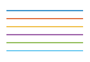
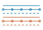
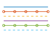
The examples in this table were created using the default colors in the ColorOrder property and three line styles (["-","-o","--"]) in the LineStyleOrder property.

Value	Description	Example
"aftercolor"	Cycle through the line styles of the LineStyleOrder after the colors of the ColorOrder.
"beforecolor"	Cycle through the line styles of the LineStyleOrder before the colors of the ColorOrder.
"withcolor"	Cycle through the line styles of the LineStyleOrder with the colors of the ColorOrder.

NextSeriesIndex — SeriesIndex value for next object

Read-only: whole number

This property is read-only.

SeriesIndex value for the next plot object added to the axes, returned as a whole number greater than or equal to 0. This property is useful when you want to track how the objects cycle through the colors and line styles. This property maintains a count of the objects in the axes that have a numeric SeriesIndex property value. MATLAB uses it to assign a SeriesIndex value to each new object. The count starts at 1 when you create the axes, and it increases by 1 for each additional object. Thus, the count is typically n+1, where n is the number of objects in the axes.

If you manually change the ColorOrderIndex or LineStyleOrderIndex property on the axes, the value of the NextSeriesIndex property changes to 0. As a consequence, objects that have a SeriesIndex property no longer update automatically when you change the ColorOrder or LineStyleOrder properties on the axes.

NextPlot — Properties to reset

'replace' (default) | 'add' | 'replacechildren' | 'replaceall'

Properties to reset when adding a new plot to the axes, specified as one of these values:

• 'add' — Add new plots to the existing axes. Do not delete existing plots or reset axes properties before displaying the new plot.

• 'replacechildren' — Delete existing plots before displaying the new plot. Reset the ColorOrderIndex and LineStyleOrderIndex properties to 1, but do not reset other axes properties. The next plot added to the axes uses the first color and line style based on the ColorOrder and LineStyle order properties. This value is similar to using cla before every new plot.

• 'replace' — Delete existing plots and reset axes properties, except Position and Units, to their default values before displaying the new plot.

• 'replaceall' — Delete existing plots and reset axes properties, except Position and Units, to their default values before displaying the new plot. This value is similar to using cla reset before every new plot.

Note

For Axes objects with only one y-axis, the 'replace' and 'replaceall' property values are equivalent. For Axes objects with two y-axes, the 'replace' value affects only the active side while the 'replaceall' value affects both sides.

Figures also have a NextPlot property. Alternatively, you can use the newplot function to prepare figures and axes for subsequent graphics commands.

SortMethod — Order for rendering objects

'depth' | 'childorder'

Order for rendering objects, specified as one of these values:

• 'depth' — Draw objects in back-to-front order based on the current view. Use this value to ensure that objects in front of other objects are drawn correctly.

• 'childorder' — Draw objects in the order in which they are created by graphics functions, without considering the relationship of the objects in three dimensions. This value can result in faster rendering, particularly if the figure is very large, but also can result in improper depth sorting of the objects displayed.

LineStyleOrderIndex — Line style order index

1 (default) | positive integer

Line style order index, specified as a positive integer. This property specifies the next line style MATLAB selects from the axes LineStyleOrder property to create the next plot line.

Note

Setting the SeriesIndex property of individual plot objects is recommended over setting the LineStyleOrderIndex property of the axes. The behavior of the LineStyleOrderIndex property changed in R2019b. For more information, see Indexing scheme for ColorOrder and LineStyleOrder might change plot colors and line styles.

Color and Transparency Maps

Colormap — Color map

parula (default) | m-by-3 array of RGB triplets

Color map, specified as an m-by-3 array of RGB (red, green, blue) triplets that define m individual colors.

Example: ax.Colormap = [1 0 1; 0 0 1; 1 1 0] sets the color map to three colors: magenta, blue, and yellow.

MATLAB accesses these colors by their row number.

Alternatively, use the colormap function to change the color map.

ColorScale — Scale for color mapping

'linear' (default) | 'log'

Scale for color mapping, specified as one of these values:

• 'linear' — Linear scale. The tick values along the colorbar also use a linear scale.

• 'log' — Log scale. The tick values along the colorbar also use a log scale.

CLim — Color limits for colormap

[0 1] (default) | two-element vector of the form [cmin cmax]

Color limits for the colormap, specified as a two-element vector of the form [cmin cmax].

If the associated mode property is set to 'auto', then MATLAB chooses the color limits. If you assign a value to this property, then MATLAB sets the mode to 'manual' and does not automatically choose the color limits.

CLimMode — Selection mode for CLim

'auto' (default) | 'manual'

Selection mode for the CLim property, specified as one of these values:

• 'auto' — Automatically select the limits based on the color data of the graphics objects contained in the axes.

• 'manual' — Manually specify the values. To specify the values, set the CLim property. The values do not change when the limits of the axes children change.

Alphamap — Transparency map

array of 64 values from 0 to 1 (default) | array of finite alpha values from 0 to 1

Transparency map, specified as an array of finite alpha values that progress linearly from 0 to 1. The size of the array can be m-by-1 or 1-by-m. MATLAB accesses alpha values by their index in the array. An alphamap can be any length.

AlphaScale — Scale for transparency mapping

'linear' (default) | 'log'

Scale for transparency mapping, specified as one of these values:

• 'linear' — Linear scale

• 'log' — Log scale

ALim — Alpha limits for alphamap

[0 1] (default) | two-element vector of the form [amin amax]

Alpha limits for alphamap, specified as a two-element vector of the form [amin amax].

If the associated mode property is set to 'auto', then MATLAB chooses the alpha limits. If you set this property, then MATLAB sets the mode to 'manual' and does not automatically choose the alpha limits.

ALimMode — Selection mode for ALim

'auto' (default) | 'manual'

Selection mode for the ALim property, specified as one of these values:

• 'auto' — Automatically select the limits based on the AlphaData values of the graphics objects contained in the axes.

• 'manual' — Manually specify the alpha limits. To specify the alpha limits, set the ALim property.

Box Styling

Color — Background color

RGB triplet | hexadecimal color code | 'r' | 'g' | 'b' | ...

Background color, specified as an RGB triplet, a hexadecimal color code, a color name, or a short name.

For a custom color, specify an RGB triplet or a hexadecimal color code.

• An RGB triplet is a three-element row vector whose elements specify the intensities of the red, green, and blue components of the color. The intensities must be in the range [0,1], for example, [0.4 0.6 0.7].

• A hexadecimal color code is a string scalar or character vector that starts with a hash symbol (#) followed by three or six hexadecimal digits, which can range from 0 to F. The values are not case sensitive. Therefore, the color codes "#FF8800", "#ff8800", "#F80", and "#f80" are equivalent.

Alternatively, you can specify some common colors by name. This table lists the named color options, the equivalent RGB triplets, and the hexadecimal color codes.

Color Name	Short Name	RGB Triplet	Hexadecimal Color Code	Appearance
"red"	"r"	[1 0 0]	"#FF0000"
"green"	"g"	[0 1 0]	"#00FF00"
"blue"	"b"	[0 0 1]	"#0000FF"
"cyan"	"c"	[0 1 1]	"#00FFFF"
"magenta"	"m"	[1 0 1]	"#FF00FF"
"yellow"	"y"	[1 1 0]	"#FFFF00"
"black"	"k"	[0 0 0]	"#000000"
"white"	"w"	[1 1 1]	"#FFFFFF"
"none"	Not applicable	Not applicable	Not applicable	No color

This table lists the default color palettes for plots in the light and dark themes.

Palette	Palette Colors
"gem" — Light theme default Before R2025a: Most plots use these colors by default.
"glow" — Dark theme default

You can get the RGB triplets and hexadecimal color codes for these palettes using the orderedcolors and rgb2hex functions. For example, get the RGB triplets for the "gem" palette and convert them to hexadecimal color codes.

RGB = orderedcolors("gem");
H = rgb2hex(RGB);

Before R2023b: Get the RGB triplets using RGB = get(groot,"FactoryAxesColorOrder").

Before R2024a: Get the hexadecimal color codes using H = compose("#%02X%02X%02X",round(RGB*255)).

Example: ax.Color = 'none'

LineWidth — Width of circular and angle lines

0.5 (default) | scalar value

Width of circular and angle lines, specified as a scalar value in point units. One point equals 1/72 inch.

Example: ax.LineWidth = 1.5

Box — Outline around polar axes

'off' (default) | on/off logical value

Outline around the polar axes, specified as 'on' or 'off', or as numeric or logical 1 (true) or 0 (false). A value of 'on' is equivalent to true, and 'off' is equivalent to false. Thus, you can use the value of this property as a logical value. The value is stored as an on/off logical value of type matlab.lang.OnOffSwitchState.

The difference between the values is most noticeable when the theta-axis limits do not span 360 degrees.

Value	Result
'on'	Display the full outline around the polar axes.
'off'	Do not display the full outline around the polar axes.

Example: ax.Box = 'on'

Clipping — Clipping of objects to polar axes boundary

'on' (default) | on/off logical value

Clipping of objects to the polar axes boundary, specified as 'on' or 'off', or as numeric or logical 1 (true) or 0 (false). A value of 'on' is equivalent to true, and 'off' is equivalent to false. Thus, you can use the value of this property as a logical value. The value is stored as an on/off logical value of type matlab.lang.OnOffSwitchState.

The clipping behavior of an object in the polar axes depends on both the Clipping property of the polar axes and the Clipping property of the individual object. The property value of the polar axes has these effects:

• 'on' — Allow each individual object in the polar axes to control its own clipping behavior based on the Clipping property value for the object.

• 'off' — Disable clipping for all objects in the polar axes, regardless of the Clipping property value for the individual objects. Parts of objects can appear outside of the polar axes limits. For example, parts can appear outside the limits if you create a plot, set hold on, freeze the axis scaling, and then add a plot that is larger than the original plot.

This table lists the results for different combinations of Clipping property values.

Clipping Property for Axes Object	Clipping Property for Individual Object	Result
'on'	'on'	Individual object is clipped. Others might or might not be.
'on'	'off'	Individual object is not clipped. Others might or might not be.
'off'	'on'	Individual object and other objects are not clipped.
'off'	'off'	Individual object and other objects are not clipped.

Thick lines and markers might display outside the polar axes limits, even if clipping is enabled. If a plot contains markers, then as long as the data point lies within the polar axes, MATLAB draws the entire marker.

Position

OuterPosition — Size and position of polar axes, including labels and margins

[0 0 1 1] (default) | four-element vector

Size and position of polar axes, including the labels and margins, specified as a four-element vector of the form [left bottom width height]. This vector defines the extents of the rectangle that encloses the outer bounds of the polar axes. The left and bottom elements define the distance from the lower-left corner of the figure or uipanel that contains the polar axes to the lower-left corner of the rectangle. The width and height elements are the rectangle dimensions.

By default, the values are measured in units normalized to the container. To change the units, set the Units property. The default value of [0 0 1 1] includes the whole interior of the container.

Note

Setting this property has no effect when the parent container is a TiledChartLayout object.

InnerPosition — Inner size and location

[0.1300 0.1100 0.7750 0.8150] (default) | four-element vector

Inner size and location, specified as a four-element vector of the form [left bottom width height]. This property is equivalent to the Position property.

Note

• When querying the inner position, consider using the tightPosition function for more accuracy. (since R2022b)

• Setting this property has no effect when the parent container is a TiledChartLayout

Position — Size and location of polar axes, not including labels or margins

[0.1300 0.1100 0.7750 0.8150] (default) | four-element vector

Size and location of the polar axes, not including labels or margins, specified as a four-element vector of the form [left bottom width height]. This vector defines the extents of the tightest bounding rectangle that encloses the polar axes. The left and bottom elements define the distance from the lower-left corner of the container to the lower-left corner of the rectangle. The width and height elements are the rectangle dimensions.

By default, the values are measured in units normalized to the container. To change the units, set the Units property.

Example: ax.Position = [0 0 1 1]

Note

• When querying the position, consider using the tightPosition function for more accuracy. (since R2022b)

• Setting this property has no effect when the parent container is a TiledChartLayout

TightInset — Margins for text labels

Read-only: four-element vector of the form [left bottom right top]

This property is read-only.

Margins for the text labels, returned as a four-element vector of the form [left bottom right top]. The elements define the distances between the bounds of the Position property and the extent of the polar axes text labels and title. By default, the values are measured in units normalized to the figure or uipanel that contains the polar axes. To change the units, set the Units property.

The Position property and the TightInset property define the tightest bounding box that encloses the polar axes and its labels and title.

PositionConstraint — Position to hold constant

"outerposition" | "innerposition"

Position property to hold constant when adding, removing, or changing decorations, specified as one of the following values:

• "outerposition" — The OuterPosition property remains constant when you add, remove, or change decorations such as a title or an axis label. If any positional adjustments are needed, MATLAB adjusts the InnerPosition property.

• "innerposition" — The InnerPosition property remains constant when you add, remove, or change decorations such as a title or an axis label. If any positional adjustments are needed, MATLAB adjusts the OuterPosition property.

Note

Setting this property has no effect when the parent container is a TiledChartLayout object.

Units — Position units

"normalized" (default) | "inches" | "centimeters" | "points" | "pixels" | "characters"

Position units, specified as one of these values.

Units	Description
"normalized" (default)	Normalized with respect to the container, which is typically the figure or a panel. The lower left corner of the container maps to (0,0) and the upper right corner maps to (1,1).
"inches"	Inches.
"centimeters"	Centimeters.
"characters"	Based on the default uicontrol font of the graphics root object: Character width = width of letter x. Character height = distance between the baselines of two lines of text.
"points"	Typography points. One point equals 1/72 inch.
"pixels"	Pixels. On Windows and Macintosh systems, the size of a pixel is 1/96th of an inch. This size is independent of your system resolution. On Linux systems, the size of a pixel is determined by your system resolution.

When specifying the units as a Name,Value pair during object creation, you must set the Units property before specifying the properties that you want to use these units, such as Position.

Layout — Layout options

empty LayoutOptions array (default) | TiledChartLayoutOptions object | GridLayoutOptions object

Layout options, specified as a TiledChartLayoutOptions or a GridLayoutOptions object. This property is useful when the axes object is either in a tiled chart layout or a grid layout.

To position the axes within the grid of a tiled chart layout, set the Tile and TileSpan properties on the TiledChartLayoutOptions object. For example, consider a 3-by-3 tiled chart layout. The layout has a grid of tiles in the center, and four tiles along the outer edges. In practice, the grid is invisible and the outer tiles do not take up space until you populate them with axes or charts.

This code places the axes ax in the third tile of the grid.

ax.Layout.Tile = 3;

To make the axes span multiple tiles, specify the TileSpan property as a two-element vector. For example, this axes spans 2 rows and 3 columns of tiles.

ax.Layout.TileSpan = [2 3];

To place the axes in one of the surrounding tiles, specify the Tile property as 'north', 'south', 'east', or 'west'. For example, setting the value to 'east' places the axes in the tile to the right of the grid.

ax.Layout.Tile = 'east';

To place the axes into a layout within an app, specify this property as a GridLayoutOptions object. For more information about working with grid layouts in apps, see uigridlayout.

If the axes is not a child of either a tiled chart layout or a grid layout (for example, if it is a child of a figure or panel) then this property is empty and has no effect.

Interactivity

InteractionOptions — Options to customize interaction behavior

PolarAxesInteractionOptions object

Since R2024a

Options to customize interaction behavior, specified as a PolarAxesInteractionOptions object. Use the properties of the PolarAxesInteractionOptions object to customize the behavior of interactions with the polar axes. For a complete list of properties, see PolarAxesInteractionOptions Properties.

The options set by the PolarAxesInteractionOptions object apply to these interactions on the associated polar axes:

• The built-in interactions specified by the Interactions property of the polar axes

• Interactions enabled by using mode functions, such as datacursormode

• Interactions enabled using the polar axes toolbar

Example: pax.InteractionOptions.DatatipsPlacementMethod = "interpolate" allows data tips to be placed at locations on the plot that are between data points.

Toolbar — Data exploration toolbar

AxesToolbar object (default)

Data exploration toolbar, which is an AxesToolbar object. The toolbar appears at the top-right corner of the axes when you hover over it and includes options for exporting and data tips.

You can customize the toolbar buttons using the axtoolbar and axtoolbarbtn functions.

If you do not want the toolbar to appear when you hover over the axes, set the Visible property of the AxesToolbar object to 'off'.

ax = gca;
ax.Toolbar.Visible = 'off';

For more information, see AxesToolbar Properties.

Interactions — Interactions

DataTipInteraction object (default) | []

Interactions, specified as a DataTipInteraction object or an empty array. When the value of this property is a DataTipInteraction object, you can display data tips within your chart without selecting any of the axes toolbar buttons.

To remove all interactions from the axes, set this property to an empty array. To temporarily disable the current set of interactions, call the disableDefaultInteractivity function. You can reenable them by calling the enableDefaultInteractivity function.

Note

The DataTipInteraction object is not returned by findobj or findall, and it is not copied by copyobj.

For more information about chart interactions, see Control Chart Interactivity.

Visible — State of visibility

'on' (default) | on/off logical value

State of visibility, specified as 'on' or 'off', or as numeric or logical 1 (true) or 0 (false). A value of 'on' is equivalent to true, and 'off' is equivalent to false. Thus, you can use the value of this property as a logical value. The value is stored as an on/off logical value of type matlab.lang.OnOffSwitchState.

• 'on' — Display the axes and its children.

• 'off' — Hide the axes without deleting it. You still can access the properties of an invisible axes object.

Note

When the Visible property is 'off', the axes object is invisible, but child objects such as lines remain visible.

CurrentPoint — Location of mouse pointer

Read-only: two-element vector

This property is read-only.

Location of mouse pointer, returned as a two element vector of the form [th r]. The elements of the vector indicate the location of the last click within the axes. th is the theta angle in radians, and r is the radius value. Each value is bounded by the following limits:

• The theta angle is in the range [tmin, tmin+2*pi], where tmin is the first value of the ThetaLim vector of the polar axes. The angle is measured from the location of the zero angle in the direction specified by the ThetaDir property. The location of the zero angle is specified by the ThetaZeroLocation property. By default, the zero angle on the right side of the axes, and the direction is counterclockwise.

• The radius value is greater than or equal to rmin, where rmin is the first value in the RLim vector of the polar axes.

If the figure has a WindowButtonMotionFcn callback defined, then the value indicates the last location of the pointer. The figure also has a CurrentPoint property.

ContextMenu — Context menu

empty GraphicsPlaceholder array (default) | ContextMenu object

Context menu, specified as a ContextMenu object. Use this property to display a context menu when you right-click the object. Create the context menu using the uicontextmenu function.

Note

If the PickableParts property is set to 'none' or if the HitTest property is set to 'off', then the context menu does not appear.

Selected — Selection state

'off' (default) | on/off logical value

Selection state, specified as 'on' or 'off', or as numeric or logical 1 (true) or 0 (false). A value of 'on' is equivalent to true, and 'off' is equivalent to false. Thus, you can use the value of this property as a logical value. The value is stored as an on/off logical value of type matlab.lang.OnOffSwitchState.

• 'on' — Selected. If you click the object when in plot edit mode, then MATLAB sets its Selected property to 'on'. If the SelectionHighlight property also is set to 'on', then MATLAB displays selection handles around the object.

• 'off' — Not selected.

SelectionHighlight — Display of selection handles

'on' (default) | on/off logical value

Display of selection handles when selected, specified as 'on' or 'off', or as numeric or logical 1 (true) or 0 (false). A value of 'on' is equivalent to true, and 'off' is equivalent to false. Thus, you can use the value of this property as a logical value. The value is stored as an on/off logical value of type matlab.lang.OnOffSwitchState.

• 'on' — Display selection handles when the Selected property is set to 'on'.

• 'off' — Never display selection handles, even when the Selected property is set to 'on'.

Callbacks

ButtonDownFcn — Mouse-click callback

'' (default) | function handle | cell array | character vector

Mouse-click callback, specified as one of these values:

• Function handle

• Cell array containing a function handle and additional arguments

• Character vector that is a valid MATLAB command or function, which is evaluated in the base workspace (not recommended)

Use this property to execute code when you click the object. If you specify this property using a function handle, then MATLAB passes two arguments to the callback function when executing the callback:

• Clicked object — Access properties of the clicked object from within the callback function.

• Event data — Empty argument. Replace it with the tilde character (~) in the function definition to indicate that this argument is not used.

For more information on how to use function handles to define callback functions, see Create Callbacks for Graphics Objects.

Note

If the PickableParts property is set to 'none' or if the HitTest property is set to 'off', then this callback does not execute.

CreateFcn — Creation function

'' (default) | function handle | cell array | character vector

Object creation function, specified as one of these values:

• Function handle.

• Cell array in which the first element is a function handle. Subsequent elements in the cell array are the arguments to pass to the callback function.

• Character vector containing a valid MATLAB expression (not recommended). MATLAB evaluates this expression in the base workspace.

For more information about specifying a callback as a function handle, cell array, or character vector, see Create Callbacks for Graphics Objects.

This property specifies a callback function to execute when MATLAB creates the object. MATLAB initializes all property values before executing the CreateFcn callback. If you do not specify the CreateFcn property, then MATLAB executes a default creation function.

Setting the CreateFcn property on an existing component has no effect.

If you specify this property as a function handle or cell array, you can access the object that is being created using the first argument of the callback function. Otherwise, use the gcbo function to access the object.

DeleteFcn — Deletion function

'' (default) | function handle | cell array | character vector

Object deletion function, specified as one of these values:

• Function handle.

• Cell array in which the first element is a function handle. Subsequent elements in the cell array are the arguments to pass to the callback function.

• Character vector containing a valid MATLAB expression (not recommended). MATLAB evaluates this expression in the base workspace.

For more information about specifying a callback as a function handle, cell array, or character vector, see Create Callbacks for Graphics Objects.

This property specifies a callback function to execute when MATLAB deletes the object. MATLAB executes the DeleteFcn callback before destroying the properties of the object. If you do not specify the DeleteFcn property, then MATLAB executes a default deletion function.

If you specify this property as a function handle or cell array, you can access the object that is being deleted using the first argument of the callback function. Otherwise, use the gcbo function to access the object.

Callback Execution Control

Interruptible — Callback interruption

'on' (default) | on/off logical value

Callback interruption, specified as 'on' or 'off', or as numeric or logical 1 (true) or 0 (false). A value of 'on' is equivalent to true, and 'off' is equivalent to false. Thus, you can use the value of this property as a logical value. The value is stored as an on/off logical value of type matlab.lang.OnOffSwitchState.

This property determines if a running callback can be interrupted. There are two callback states to consider:

• The running callback is the currently executing callback.

• The interrupting callback is a callback that tries to interrupt the running callback.

MATLAB determines callback interruption behavior whenever it executes a command that processes the callback queue. These commands include drawnow, figure, uifigure, getframe, waitfor, and pause.

If the running callback does not contain one of these commands, then no interruption occurs. MATLAB first finishes executing the running callback, and later executes the interrupting callback.

If the running callback does contain one of these commands, then the Interruptible property of the object that owns the running callback determines if the interruption occurs:

• If the value of Interruptible is 'off', then no interruption occurs. Instead, the BusyAction property of the object that owns the interrupting callback determines if the interrupting callback is discarded or added to the callback queue.

• If the value of Interruptible is 'on', then the interruption occurs. The next time MATLAB processes the callback queue, it stops the execution of the running callback and executes the interrupting callback. After the interrupting callback completes, MATLAB then resumes executing the running callback.

Note

Callback interruption and execution behave differently in these situations:

• If the interrupting callback is a DeleteFcn, CloseRequestFcn, or SizeChangedFcn callback, then the interruption occurs regardless of the Interruptible property value.

• If the running callback is currently executing the waitfor function, then the interruption occurs regardless of the Interruptible property value.

• If the interrupting callback is owned by a Timer object, then the callback executes according to schedule regardless of the Interruptible property value.

Note

When an interruption occurs, MATLAB does not save the state of properties or the display. For example, the object returned by the gca or gcf command might change when another callback executes.

BusyAction — Callback queuing

'queue' (default) | 'cancel'

Callback queuing, specified as 'queue' or 'cancel'. The BusyAction property determines how MATLAB handles the execution of interrupting callbacks. There are two callback states to consider:

• The running callback is the currently executing callback.

• The interrupting callback is a callback that tries to interrupt the running callback.

The BusyAction property determines callback queuing behavior only when both of these conditions are met:

• The running callback contains a command that processes the callback queue, such as drawnow, figure, uifigure, getframe, waitfor, or pause.

• The value of the Interruptible property of the object that owns the running callback is 'off'.

Under these conditions, the BusyAction property of the object that owns the interrupting callback determines how MATLAB handles the interrupting callback. These are possible values of the BusyAction property:

• 'queue' — Puts the interrupting callback in a queue to be processed after the running callback finishes execution.

• 'cancel' — Does not execute the interrupting callback.

PickableParts — Ability to capture mouse clicks

'visible' (default) | 'all' | 'none'

Ability to capture mouse clicks, specified as one of these values:

• 'visible' — Capture mouse clicks only when visible. The Visible property must be set to 'on'. The HitTest property determines if the PolarAxes object responds to the click or if an ancestor does.

• 'all' — Capture mouse clicks regardless of visibility. The Visible property can be set to 'on' or 'off'. The HitTest property determines if the PolarAxes object responds to the click or if an ancestor does.

• 'none' — Cannot capture mouse clicks. Clicking the PolarAxes object passes the click to the object below it in the current view of the figure window, which is typically the axes or the figure. The HitTest property has no effect.

If you want an object to be clickable when it is underneath other objects that you do not want to be clickable, then set the PickableParts property of the other objects to 'none' so that the click passes through them.

HitTest — Response to captured mouse clicks

'on' (default) | on/off logical value

Response to captured mouse clicks, specified as 'on' or 'off', or as numeric or logical 1 (true) or 0 (false). A value of 'on' is equivalent to true, and 'off' is equivalent to false. Thus, you can use the value of this property as a logical value. The value is stored as an on/off logical value of type matlab.lang.OnOffSwitchState.

• 'on' — Trigger the ButtonDownFcn callback of the PolarAxes object. If you have defined the ContextMenu property, then invoke the context menu.

• 'off' — Trigger the callbacks for the nearest ancestor of the PolarAxes object that meets one of these conditions:

  • HitTest property is set to 'on'.

  • PickableParts property is set to a value that enables the ancestor to capture mouse clicks.

Note

The PickableParts property determines if the PolarAxes object can capture mouse clicks. If it cannot, then the HitTest property has no effect.

BeingDeleted — Deletion status

Read-only: on/off logical value

This property is read-only.

Deletion status, returned as an on/off logical value of type matlab.lang.OnOffSwitchState.

MATLAB sets the BeingDeleted property to 'on' when the DeleteFcn callback begins execution. The BeingDeleted property remains set to 'on' until the component object no longer exists.

Check the value of the BeingDeleted property to verify that the object is not about to be deleted before querying or modifying it.

Parent/Child

Parent — Parent container

Figure object | Panel object | Tab object | TiledChartLayout object | GridLayout object

Parent container, specified as a Figure, Panel, Tab, TiledChartLayout, or GridLayout object.

Children — Children

empty GraphicsPlaceholder array | array of graphics objects

Children, returned as an array of graphics objects. Use this property to view a list of the children or to reorder the children by setting the property to a permutation of itself.

You cannot add or remove children using the Children property. To add a child to this list, set the Parent property of the child graphics object to the PolarAxes object.

HandleVisibility — Visibility of object handle

"on" (default) | "off" | "callback"

Visibility of the object handle in the Children property of the parent, specified as one of these values:

• "on" — Object handle is always visible.

• "off" — Object handle is invisible at all times. This option is useful for preventing unintended changes by another function. Set HandleVisibility to "off" to temporarily hide the handle during the execution of that function.

• "callback" — Object handle is visible from within callbacks or functions invoked by callbacks, but not from within functions invoked from the command line. This option blocks access to the object at the command line, but permits callback functions to access it.

If the object is not listed in the Children property of the parent, then functions that obtain object handles by searching the object hierarchy or querying handle properties cannot return it. Examples of such functions include the get, findobj, gca, gcf, gco, newplot, cla, clf, and close functions.

Hidden object handles are still valid. Set the root ShowHiddenHandles property to "on" to list all object handles regardless of their HandleVisibility property setting.

Identifiers

Type — Type of graphics object

Read-only: 'polaraxes' (default)

This property is read-only.

Type of graphics object, returned as 'polaraxes'.

Tag — Object identifier

'' (default) | character vector | string scalar

Object identifier, specified as a character vector or string scalar. You can specify a unique Tag value to serve as an identifier for an object. When you need access to the object elsewhere in your code, you can use the findobj function to search for the object based on the Tag value.

UserData — User data

[] (default) | array

User data, specified as any MATLAB array. For example, you can specify a scalar, vector, matrix, cell array, character array, table, or structure. Use this property to store arbitrary data on an object.

If you are working in App Designer, create public or private properties in the app to share data instead of using the UserData property. For more information, see Share Data Within App Designer Apps.

Version History

Introduced before R2006a

R2025a: Default plot colors and tick label colors have changed slightly

The default ColorOrder, RColor, and ThetaColor property values in the light theme have changed slightly. This table lists the changes.

Property	R2024b Color	R2025a Color
ColorOrder	RGB Triplet Sample [0.0000 0.4470 0.7410] [0.8500 0.3250 0.0980] [0.9290 0.6940 0.1250] [0.4940 0.1840 0.5560] [0.4660 0.6740 0.1880] [0.3010 0.7450 0.9330] [0.6350 0.0780 0.1840]	RGB Triplet Sample [0.0660 0.4430 0.7450] [0.8660 0.3290 0.0000] [0.9290 0.6940 0.1250] [0.5210 0.0860 0.8190] [0.2310 0.6660 0.1960] [0.1840 0.7450 0.9370] [0.8190 0.0150 0.5450]
RColor and ThetaColor	[0.15 0.15 0.15]	[0.1294 0.1294 0.1294]

R2025a: Specify the location of zero degrees as an angle using the ThetaZeroLocation property

Specify the location of zero degrees as an angle value by setting the ThetaZeroAxisLocaton property to a value such as 45 (when the ThetaAxisUnits property is "degrees") or pi/4 when the ThetaAxisUnits property is "radians").

The existing options, "right", "left", "top" and "bottom", are also supported.

R2025a: FontSmoothing property has no effect

The FontSmoothing property has no effect and will be removed in a future release. You can set or get the value of this property without warning, but all text is smooth regardless of the property value. This property removal was announced in R2022a.

R2024a: Customize behavior of interactions using the InteractionOptions property

For polaraxes objects created in App Designer or in figures created using the uifigure function, you can customize the behavior of axes interactions. Customize the behavior of data tips by using the InteractionOptions property.

R2023a: Control cycling of line styles using the LineStyleCyclingMethod property

Use the LineStyleCyclingMethod property to control how different lines are distinguished from one another in the axes.

R2022a: Control tick label rotation using the RTickLabelRotationMode property

Now you can control the selection mode for the r-axis tick label rotation by setting the RTickLabelRotationMode property.

R2021b: Remove tick marks by setting the TickDir property to "none"

You can remove all the tick marks from the axes by setting the TickDir property to "none".

R2020b: Control the alignment of a plot title with the TitleHorizontalAlignment property

You can control the alignment of a plot title by setting the TitleHorizontalAlignment property of the axes to "left", "right", or "center".

R2020b: Create and style subtitles with the Subtitle and SubtitleFontWeight properties

Add a subtitle to your plot by setting the Subtitle property or calling the subtitle function. To control the appearance of the subtitle, set the SubtitleFontWeight property.

R2020a: Preserve inner or outer position with the PositionConstraint property

Set the PositionConstraint property of a PolarAxes object to control the space around the axes when you add or modify decorations such as titles and axis labels.

R2020a: ActivePositionProperty is not recommended

Setting or getting ActivePositionProperty is not recommended. Use the PositionConstraint property instead.

There are no plans to remove ActivePositionProperty, but the property is no longer listed when you call the set, get, or properties functions on the axes.

To update your code, make these changes:

• Replace all instances of ActivePositionProperty with PositionConstraint.

• Replace all references to the 'position' option with the 'innerposition' option.

R2020a: UIContextMenu property is not recommended

Setting or getting UIContextMenu property is not recommended. Instead, use the ContextMenu property, which accepts the same type of input and behaves the same way as the UIContextMenu property.

There are no plans to remove the UIContextMenu property, but it is no longer listed when you call the set, get, or properties functions on the PolarAxes object.

R2019b: Position axes within tiled chart layouts using the Layout property

Use the Layout property to position a PolarAxes object within a tiled chart layout.

R2019b: Changing ColorOrder or LineStyleOrder affects existing plots immediately

If you change the axes ColorOrder or LineStyleOrder properties after plotting into the axes, the colors and line styles in your plot update immediately. In R2019a and previous releases, the new colors and line styles affect only subsequent plots, not the existing plots.

To preserve the original behavior, set the axes ColorOrderIndex or LineStyleOrderIndex property to any value (such as its current value) before changing the ColorOrder or LineStyleOrder property.

R2019b: Indexing scheme for ColorOrder and LineStyleOrder might change plot colors and line styles

There is a new indexing scheme that enables you to change the colors and line styles of existing plots by setting the ColorOrder or LineStyleOrder properties. MATLAB applies this indexing scheme to all objects that have a ColorMode, FaceColorMode, MarkerFaceColorMode, or CDataMode. As a result, your code might produce plots that cycle though the colors and line styles differently than in previous releases.

In R2019a and earlier releases, MATLAB uses a different indexing scheme which does not allow you to change the colors of existing plots.

To preserve the way your plots cycle through colors and line styles, set the axes ColorOrderIndex or LineStyleOrderIndex property to any value (such as its current value) before plotting into the axes.

R2019a: Customize chart interactions using the Interactions property

You can create a customized set of chart interactions by setting the Interactions property of the axes. These interactions are built into the axes and are available without having to select any buttons in the axes toolbar. Some types of interactions are enabled by default, depending on the content of the axes.

R2018a: Add a toolbar to the axes with the Toolbar property

Use the Toolbar property to add a toolbar to the top-right corner of the axes for quick access to data exploration tools.