Die Übersetzung dieser Seite ist veraltet. Klicken Sie hier, um die neueste Version auf Englisch zu sehen.

Entwurf eines LQR-Servoreglers in Simulink

Dieses Beispiel zeigt den Entwurf eines LQR-Servoreglers in Simulink® anhand einer Autopilot-Anwendung für Luftfahrzeuge.

Öffnen Sie das Modell für

open_system("lqrpilot")

In diesem Modell:

• Der Block Linearized Dynamics enthält das linearisierte Flugwerk.

• sf_aerodyn ist ein S-Function-Block, der die nichtlinearen Gleichungen für $\left(\theta ,\varphi \right)=\left(0,{15}^{\circ }\right)$ enthält.

• Das Fehlersignal zwischen $\varphi$ und ${\varphi }_{\mathrm{ref}}$ wird durch einen Integrator geschickt, der dazu beiträgt, den Fehler auf Null zu bringen.

Beim Öffnen des Modells wird auch die MAT-Datei lqrpilotData geladen, welche folgende Daten enthält:

• Matrizen der Zustandsgleichungen A und B

• Linearisierte Zustandsmatrix A15

• Endgültige LQG-Verstärkungsmatrix K_lqr

Zustandsraumgleichungen für Luftfahrzeuge

Die Gleichung ist die Standard-Zustandsgleichung eines Zustandsraumsystems.

$$\dot{\mathit{x}}=\mathit{A}\mathit{x}+\mathit{B}\mathit{u}$$

Für das Luftfahrzeugsystem sieht der Zustandsvektor wie folgt aus:

$$\mathit{x}={\left[\mathit{u},\mathit{v},\mathit{w},\mathit{p},\mathit{q},\mathit{r},\theta ,\varphi \right]}^{\mathit{T}}$$

Die Variablen $\mathit{u}$, $\mathit{v}$ und $\mathit{w}$ sind die drei Geschwindigkeiten relativ zum Flugzeugrumpf-Bezugssystem, wie in der folgenden Abbildung dargestellt.

Die Variablen $\varphi$ und $\theta$ stellen das Rollen und Nicken dar $\mathit{p}$, $\mathit{q}$ und $\mathit{r}$ sind die entsprechenden Roll-, Nick- und Giergeschwindigkeiten.

Die Dynamiken des Flugwerks sind nichtlinear. Die folgende Gleichung zeigt die Zustandsraumgleichung, nachdem die nichtlinearen Komponenten hinzugefügt wurden, wobei $\mathit{g}$ die Fallbeschleunigung ist.

$$\dot{\mathit{x}}=\mathit{Ax}+\mathit{Bu}+\left[\begin{array}{c}-\mathit{g}\cdot \sin \theta \\ \mathit{g}\cdot \cos \theta \cdot \sin \varphi \\ \mathit{g}\cdot \cos \theta \cdot \cos \varphi \\ 0\\ 0\\ 0\\ \mathit{q}\cdot \cos \varphi -\mathit{r}\cdot \sin \varphi \\ \left(\mathit{q}\cdot \sin \varphi +\mathit{r}\cdot \cos \varphi \right)\cdot \tan \theta \end{array}\right]$$

Trimmen

Für LQG-Entwurfszwecke werden die nichtlinearen Dynamiken bei $\varphi ={15}^{\circ }$ getrimmt und $\mathit{p}$, $\mathit{q}$, $\mathit{r}$ und $\theta$ auf null festgelegt. Da $\mathit{u}$, $\mathit{v}$ und $\mathit{w}$ nicht auf den nichtlinearen Term in der vorstehenden Gleichung auswirken, ist das Ergebnis ein um $\left(\theta ,\varphi \right)=\left(0,{15}^{\circ }\right)$ linearisiertes Modell, bei dem alle restlichen Zustände auf null festgelegt sind.

Das lqrdes-Skript beschreibt, wie das linearisierte Modell A15 an diesem getrimmten Arbeitspunkt berechnet wird.

Problemdefinition

Das Ziel des Entwurfs besteht im Fliegen einer stabil koordinierten Wende, wie in der folgenden Abbildung dargestellt.

Um dieses Ziel zu erreichen, müssen Sie eine Steuerung entwerfen, die eine stabile Wende beherrscht, indem eine 60-Grad-Rolle durchlaufen wird. Zusätzlich muss vorausgesetzt werden, dass der Nickwinkel $\theta$ möglichst nahe bei Null bleiben muss.

Ergebnisse

Das lqrdes-Skript beschreibt, wie die LQG-Verstärkungsmatrix K_lqr berechnet wird.

Stellen Sie im lqrpilot-Modell sicher, dass der Schalterblock so konfiguriert ist, dass er den Ausgang des Blocks „Nonlinear Dynamics“ wählt.

Führen Sie das Modell aus.

sim("lqrpilot")

Betrachten Sie die Antwort des Rollens $\varphi$ auf eine Sprungänderung von 60°. Das System verfolgt die befohlene Rolle innerhalb von etwa 60 Sekunden.

open_system("lqrpilot/phi (roll angle)")

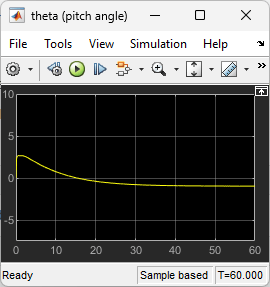
Betrachten Sie den Nickwinkel $\theta$. Der Regler war in der Lage, den Nickwinkel relativ klein zu halten.

open_system("lqrpilot/theta (pitch angle)")

Sehen Sie sich schließlich die Steuerungseingänge an.

open_system("lqrpilot/Control Inputs")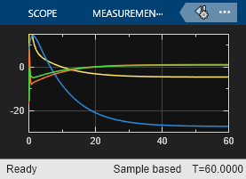

Sie können die Q- und R-Werte im lqrdes-Skript anpassen, um verschiedene mögliche Entwürfe auszuprobieren. Außerdem können Sie Simulationen der linearen und nichtlinearen Systemdynamiken vergleichen, um die Auswirkungen der Nichtlinearitäten auf die Systemleistung zu sehen.

Verwandte Themen

• Kalman-Filterung
• Entwurf von linear-quadratischen Gauß-Regelungen (LQG-Entwurf)
• Entwurf eines LQG-Reglers
• Entwurf eines LQG-Servoreglers