iopzmap

Plot pole-zero map for I/O pairs of model

Syntax

iopzmap(sys)
iopzmap(sys1,sys2,...)


Description

iopzmap(sys) computes and plots the poles and zeros of each input/output pair of the dynamic system model sys. The poles are plotted as x's and the zeros are plotted as o's.

iopzmap(sys1,sys2,...) shows the poles and zeros of multiple models sys1,sys2,... on a single plot. You can specify distinctive colors for each model, as in iopzmap(sys1,'r',sys2,'y',sys3,'g').

The functions sgrid or zgrid can be used to plot lines of constant damping ratio and natural frequency in the s or z plane.

For model arrays, iopzmap plots the poles and zeros of each model in the array on the same diagram.

Examples

Pole-Zero Map for MIMO System

Create a one-input, two-output dynamic system.

H = [tf(-5 ,[1 -1]); tf([1 -5 6],[1 1 0])];

Plot a pole-zero map.

iopzmap(H)

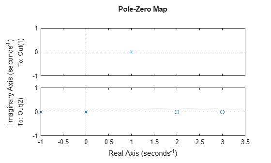
iopzmap generates a separate map for each I/O pair in the system.

Pole-Zero Map of Identified Model

View the poles and zeros of an over-parameterized state-space model estimated from input-output data. (Requires System Identification Toolbox™).

load iddata1
sys = ssest(z1,6,ssestOptions('focus','simulation'));
iopzmap(sys)

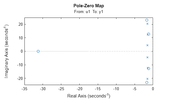
The plot shows that there are two pole-zero pairs that almost overlap, which hints are their potential redundancy.

Tips

For additional options for customizing the appearance of the pole-zero plot, use iopzplot.

Version History

Introduced in R2012a