kfoldPredict

Predict labels for observations not used for training

Syntax

Label = kfoldPredict(CVMdl)

Label = kfoldPredict(CVMdl,Name,Value)

[Label,NegLoss,PBScore] = kfoldPredict(___)

[Label,NegLoss,PBScore,Posterior] = kfoldPredict(___)

Description

Label = kfoldPredict(CVMdl) returns class labels predicted by the cross-validated ECOC model composed of linear classification models CVMdl. That is, for every fold, kfoldPredict predicts class labels for observations that it holds out when it trains using all other observations. kfoldPredict applies the same data used create CVMdl (see fitcecoc).

Also, Label contains class labels for each regularization strength in the linear classification models that compose CVMdl.

Label = kfoldPredict(CVMdl,Name,Value) returns predicted class labels with additional options specified by one or more Name,Value pair arguments. For example, specify the posterior probability estimation method, decoding scheme, or verbosity level.

[Label,NegLoss,PBScore] = kfoldPredict(___) additionally returns, for held-out observations and each regularization strength:

• Negated values of the average binary loss per class (NegLoss).

• Positive-class scores (PBScore) for each binary learner.

[Label,NegLoss,PBScore,Posterior] = kfoldPredict(___) additionally returns posterior class probability estimates for held-out observations and for each regularization strength. To return posterior probabilities, the linear classification model learners must be logistic regression models.

Input Arguments

CVMdl — Cross-validated, ECOC model composed of linear classification models

ClassificationPartitionedLinearECOC model object

Cross-validated, ECOC model composed of linear classification models, specified as a ClassificationPartitionedLinearECOC model object. You can create a ClassificationPartitionedLinearECOC model using fitcecoc and by:

1. Specifying any one of the cross-validation, name-value pair arguments, for example, CrossVal

2. Setting the name-value pair argument Learners to 'linear' or a linear classification model template returned by templateLinear

To obtain estimates, kfoldPredict applies the same data used to cross-validate the ECOC model (X and Y).

Name-Value Arguments

Specify optional pairs of arguments as Name1=Value1,...,NameN=ValueN, where Name is the argument name and Value is the corresponding value. Name-value arguments must appear after other arguments, but the order of the pairs does not matter.

Before R2021a, use commas to separate each name and value, and enclose Name in quotes.

BinaryLoss — Binary learner loss function

'hamming' | 'linear' | 'logit' | 'exponential' | 'binodeviance' | 'hinge' | 'quadratic' | function handle

Binary learner loss function, specified as the comma-separated pair consisting of 'BinaryLoss' and a built-in loss function name or function handle.

• This table contains names and descriptions of the built-in functions, where y_j is the class label for a particular binary learner (in the set {-1,1,0}), s_j is the score for observation j, and g(y_j,s_j) is the binary loss formula.

  Value	Description	Score Domain	g(yj,sj)
  "binodeviance"	Binomial deviance	(–∞,∞)	log[1 + exp(–2yjsj)]/[2log(2)]
  "exponential"	Exponential	(–∞,∞)	exp(–yjsj)/2
  "hamming"	Hamming	[0,1] or (–∞,∞)	[1 – sign(yjsj)]/2
  "hinge"	Hinge	(–∞,∞)	max(0,1 – yjsj)/2
  "linear"	Linear	(–∞,∞)	(1 – yjsj)/2
  "logit"	Logistic	(–∞,∞)	log[1 + exp(–yjsj)]/[2log(2)]
  "quadratic"	Quadratic	[0,1]	[1 – yj(2sj – 1)]2/2

  The software normalizes the binary losses such that the loss is 0.5 when y_j = 0. Also, the software calculates the mean binary loss for each class.

• For a custom binary loss function, e.g., customFunction, specify its function handle 'BinaryLoss',@customFunction.

  customFunction should have this form

  bLoss = customFunction(M,s)

  where:

  • M is the K-by-B coding matrix stored in Mdl.CodingMatrix.

  • s is the 1-by-B row vector of classification scores.

  • bLoss is the classification loss. This scalar aggregates the binary losses for every learner in a particular class. For example, you can use the mean binary loss to aggregate the loss over the learners for each class.

  • K is the number of classes.

  • B is the number of binary learners.

  For an example of passing a custom binary loss function, see Predict Test-Sample Labels of ECOC Model Using Custom Binary Loss Function.

By default, if all binary learners are linear classification models using:

• SVM, then BinaryLoss is 'hinge'

• Logistic regression, then BinaryLoss is 'quadratic'

Example: 'BinaryLoss','binodeviance'

Data Types: char | string | function_handle

Decoding — Decoding scheme

'lossweighted' (default) | 'lossbased'

Decoding scheme that aggregates the binary losses, specified as the comma-separated pair consisting of 'Decoding' and 'lossweighted' or 'lossbased'. For more information, see Binary Loss.

Example: 'Decoding','lossbased'

NumKLInitializations — Number of random initial values

0 (default) | nonnegative integer

Number of random initial values for fitting posterior probabilities by Kullback-Leibler divergence minimization, specified as the comma-separated pair consisting of 'NumKLInitializations' and a nonnegative integer.

To use this option, you must:

• Return the fourth output argument (Posterior).

• The linear classification models that compose the ECOC models must use logistic regression learners (that is, CVMdl.Trained{1}.BinaryLearners{1}.Learner must be 'logistic').

• PosteriorMethod must be 'kl'.

For more details, see Posterior Estimation Using Kullback-Leibler Divergence.

Example: 'NumKLInitializations',5

Data Types: single | double

Options — Estimation options

[] (default) | structure array

Estimation options, specified as a structure array as returned by statset.

To invoke parallel computing you need a Parallel Computing Toolbox™ license.

Example: Options=statset(UseParallel=true)

Data Types: struct

PosteriorMethod — Posterior probability estimation method

'kl' (default) | 'qp'

Posterior probability estimation method, specified as the comma-separated pair consisting of 'PosteriorMethod' and 'kl' or 'qp'.

• To use this option, you must return the fourth output argument (Posterior) and the linear classification models that compose the ECOC models must use logistic regression learners (that is, CVMdl.Trained{1}.BinaryLearners{1}.Learner must be 'logistic').

• If PosteriorMethod is 'kl', then the software estimates multiclass posterior probabilities by minimizing the Kullback-Leibler divergence between the predicted and expected posterior probabilities returned by binary learners. For details, see Posterior Estimation Using Kullback-Leibler Divergence.

• If PosteriorMethod is 'qp', then the software estimates multiclass posterior probabilities by solving a least-squares problem using quadratic programming. You need an Optimization Toolbox™ license to use this option. For details, see Posterior Estimation Using Quadratic Programming.

Example: 'PosteriorMethod','qp'

Verbose — Verbosity level

0 (default) | 1

Verbosity level, specified as 0 or 1. Verbose controls the number of diagnostic messages that the software displays in the Command Window.

If Verbose is 0, then the software does not display diagnostic messages. Otherwise, the software displays diagnostic messages.

Example: Verbose=1

Data Types: single | double

Output Arguments

Label — Cross-validated, predicted class labels

categorical array | character array | logical matrix | numeric matrix | cell array of character vectors

Cross-validated, predicted class labels, returned as a categorical or character array, logical or numeric matrix, or cell array of character vectors.

In most cases, Label is an n-by-L array of the same data type as the observed class labels (Y) used to create CVMdl. (The software treats string arrays as cell arrays of character vectors.) n is the number of observations in the predictor data (X) and L is the number of regularization strengths in the linear classification models that compose the cross-validated ECOC model. That is, Label(i,j) is the predicted class label for observation i using the ECOC model of linear classification models that has regularization strength CVMdl.Trained{1}.BinaryLearners{1}.Lambda(j).

If Y is a character array and L > 1, then Label is a cell array of class labels.

The software assigns the predicted label corresponding to the class with the largest, negated, average binary loss (NegLoss), or, equivalently, the smallest average binary loss.

NegLoss — Cross-validated, negated, average binary losses

numeric array

Cross-validated, negated, average binary losses, returned as an n-by-K-by-L numeric matrix or array. K is the number of distinct classes in the training data and columns correspond to the classes in CVMdl.ClassNames. For n and L, see Label. NegLoss(i,k,j) is the negated, average binary loss for classifying observation i into class k using the linear classification model that has regularization strength CVMdl.Trained{1}.BinaryLoss{1}.Lambda(j).

• If Decoding is 'lossbased', then NegLoss(i,k,j) is the sum of the binary losses divided by the total number of binary learners.

• If Decoding is 'lossweighted', then NegLoss(i,k,j) is the sum of the binary losses divided by the number of binary learners for the kth class.

For more details, see Binary Loss.

PBScore — Cross-validated, positive-class scores

numeric array

Cross-validated, positive-class scores, returned as an n-by-B-by-L numeric array. B is the number of binary learners in the cross-validated ECOC model and columns correspond to the binary learners in CVMdl.Trained{1}.BinaryLearners. For n and L, see Label. PBScore(i,b,j) is the positive-class score of binary learner b for classifying observation i into its positive class, using the linear classification model that has regularization strength CVMdl.Trained{1}.BinaryLearners{1}.Lambda(j).

If the coding matrix varies across folds (that is, if the coding scheme is sparserandom or denserandom), then PBScore is empty ([]).

Posterior — Cross-validated posterior class probabilities

numeric array

Cross-validated posterior class probabilities, returned as an n-by-K-by-L numeric array. For dimension definitions, see NegLoss. Posterior(i,k,j) is the posterior probability for classifying observation i into class k using the linear classification model that has regularization strength CVMdl.Trained{1}.BinaryLearners{1}.Lambda(j).

To return posterior probabilities, CVMdl.Trained{1}.BinaryLearner{1}.Learner must be 'logistic'.

Examples

Predict k-fold Cross-Validation Labels

Load the NLP data set.

load nlpdata

X is a sparse matrix of predictor data, and Y is a categorical vector of class labels.

Cross-validate an ECOC model of linear classification models.

rng(1); % For reproducibility 
CVMdl = fitcecoc(X,Y,'Learner','linear','CrossVal','on');

CVMdl is a ClassificationPartitionedLinearECOC model. By default, the software implements 10-fold cross validation.

Predict labels for the observations that fitcecoc did not use in training the folds.

label = kfoldPredict(CVMdl);

Because there is one regularization strength in CVMdl, label is a column vector of predictions containing as many rows as observations in X.

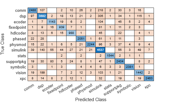
Construct a confusion matrix.

cm = confusionchart(Y,label);

Specify Custom Binary Loss

Load the NLP data set. Transpose the predictor data.

load nlpdata
X = X';

For simplicity, use the label 'others' for all observations in Y that are not 'simulink', 'dsp', or 'comm'.

Y(~(ismember(Y,{'simulink','dsp','comm'}))) = 'others';

Create a linear classification model template that specifies optimizing the objective function using SpaRSA.

t = templateLinear('Solver','sparsa');

Cross-validate an ECOC model of linear classification models using 5-fold cross-validation. Specify that the predictor observations correspond to columns.

rng(1); % For reproducibility 
CVMdl = fitcecoc(X,Y,'Learners',t,'KFold',5,'ObservationsIn','columns');
CMdl1 = CVMdl.Trained{1}

CMdl1 = 
  CompactClassificationECOC
      ResponseName: 'Y'
        ClassNames: [comm    dsp    simulink    others]
    ScoreTransform: 'none'
    BinaryLearners: {6×1 cell}
      CodingMatrix: [4×6 double]


  Properties, Methods

CVMdl is a ClassificationPartitionedLinearECOC model. It contains the property Trained, which is a 5-by-1 cell array holding a CompactClassificationECOC models that the software trained using the training set of each fold.

By default, the linear classification models that compose the ECOC models use SVMs. SVM scores are signed distances from the observation to the decision boundary. Therefore, the domain is $$(-\infty ,\infty )$$. Create a custom binary loss function that:

• Maps the coding design matrix (M) and positive-class classification scores (s) for each learner to the binary loss for each observation

• Uses linear loss

• Aggregates the binary learner loss using the median.

You can create a separate function for the binary loss function, and then save it on the MATLAB® path. Or, you can specify an anonymous binary loss function.

customBL = @(M,s)median(1 - (M.*s),2,'omitnan')/2;

Predict cross-validation labels and estimate the median binary loss per class. Print the median negative binary losses per class for a random set of 10 out-of-fold observations.

[label,NegLoss] = kfoldPredict(CVMdl,'BinaryLoss',customBL);

idx = randsample(numel(label),10);
table(Y(idx),label(idx),NegLoss(idx,1),NegLoss(idx,2),NegLoss(idx,3),...
    NegLoss(idx,4),'VariableNames',[{'True'};{'Predicted'};...
    categories(CVMdl.ClassNames)])

ans=10×6 table
      True      Predicted      comm         dsp       simulink    others 
    ________    _________    _________    ________    ________    _______

    others      others         -1.2319     -1.0488    0.048758     1.6175
    simulink    simulink       -16.407     -12.218      21.531     11.218
    dsp         dsp            -0.7387    -0.11534    -0.88466    -0.2613
    others      others         -0.1251     -0.8749    -0.99766    0.14517
    dsp         dsp             2.5867      6.4187     -3.5867    -4.4165
    others      others       -0.025358     -1.2287    -0.97464    0.19747
    others      others         -2.6725    -0.56708    -0.51092     2.7453
    others      others         -1.1605    -0.88321    -0.11679    0.43504
    others      others         -1.9511     -1.3175     0.24735    0.95111
    simulink    others          -7.848     -5.8203      4.8203     6.8457

The software predicts the label based on the maximum negated loss.

Estimate Posterior Class Probabilities

ECOC models composed of linear classification models return posterior probabilities for logistic regression learners only. This example requires the Parallel Computing Toolbox™ and the Optimization Toolbox™

Load the NLP data set and preprocess the data as in Specify Custom Binary Loss.

load nlpdata
X = X';
Y(~(ismember(Y,{'simulink','dsp','comm'}))) = 'others';

Create a set of 5 logarithmically-spaced regularization strengths from through .

Lambda = logspace(-6,-0.5,5);

Create a linear classification model template that specifies optimizing the objective function using SpaRSA and to use logistic regression learners.

t = templateLinear('Solver','sparsa','Learner','logistic','Lambda',Lambda);

Cross-validate an ECOC model of linear classification models using 5-fold cross-validation. Specify that the predictor observations correspond to columns, and to use parallel computing.

rng(1); % For reproducibility
Options = statset('UseParallel',true);
CVMdl = fitcecoc(X,Y,'Learners',t,'KFold',5,'ObservationsIn','columns',...
    'Options',Options);

Starting parallel pool (parpool) using the 'local' profile ...
Connected to the parallel pool (number of workers: 6).

Predict the cross-validated posterior class probabilities. Specify to use parallel computing and to estimate posterior probabilities using quadratic programming.

[label,~,~,Posterior] = kfoldPredict(CVMdl,'Options',Options,...
    'PosteriorMethod','qp');
size(label)
label(3,4)
size(Posterior)
Posterior(3,:,4)

ans =

       31572           5


ans = 

  categorical

     others 


ans =

       31572           4           5


ans =

    0.0285    0.0373    0.1714    0.7627

Because there are five regularization strengths:

• label is a 31572-by-5 categorical array. label(3,4) is the predicted, cross-validated label for observation 3 using the model trained with regularization strength Lambda(4).

• Posterior is a 31572-by-4-by-5 matrix. Posterior(3,:,4) is the vector of all estimated, posterior class probabilities for observation 3 using the model trained with regularization strength Lambda(4). The order of the second dimension corresponds to CVMdl.ClassNames. Display a random set of 10 posterior class probabilities.

Display a random sample of cross-validated labels and posterior probabilities for the model trained using Lambda(4).

idx = randsample(size(label,1),10);
table(Y(idx),label(idx,4),Posterior(idx,1,4),Posterior(idx,2,4),...
    Posterior(idx,3,4),Posterior(idx,4,4),...
    'VariableNames',[{'True'};{'Predicted'};categories(CVMdl.ClassNames)])

ans =

  10×6 table

      True      Predicted       comm          dsp        simulink     others  
    ________    _________    __________    __________    ________    _________

    others      others         0.030275      0.022142     0.10416      0.84342
    simulink    simulink     3.4954e-05    4.2982e-05     0.99832    0.0016016
    dsp         others          0.15787       0.25718     0.18848      0.39647
    others      others         0.094177      0.062712     0.12921      0.71391
    dsp         dsp           0.0057979       0.89703    0.015098     0.082072
    others      others         0.086084      0.054836    0.086165      0.77292
    others      others        0.0062338     0.0060492    0.023816       0.9639
    others      others          0.06543      0.075097     0.17136      0.68812
    others      others         0.051843      0.025566     0.13299       0.7896
    simulink    simulink     0.00044059    0.00049753     0.70958      0.28948

More About

Binary Loss

The binary loss is a function of the class and classification score that determines how well a binary learner classifies an observation into the class. The decoding scheme of an ECOC model specifies how the software aggregates the binary losses and determines the predicted class for each observation.

Assume the following:

• m_kj is element (k,j) of the coding design matrix M—that is, the code corresponding to class k of binary learner j. M is a K-by-B matrix, where K is the number of classes, and B is the number of binary learners.

• s_j is the score of binary learner j for an observation.

• g is the binary loss function.

• $$\widehat{k}$$ is the predicted class for the observation.

The software supports two decoding schemes:

• Loss-based decoding [3] (Decoding is "lossbased") — The predicted class of an observation corresponds to the class that produces the minimum average of the binary losses over all binary learners.

  $$\widehat{k}=\underset{k}{\text{argmin}}\frac{1}{B}{\displaystyle \sum _{j=1}^B\left|m_{kj}\right|g}(m_{kj},s_j).$$

• Loss-weighted decoding [4] (Decoding is "lossweighted") — The predicted class of an observation corresponds to the class that produces the minimum average of the binary losses over the binary learners for the corresponding class.

  $$\widehat{k}=\underset{k}{\text{argmin}}\frac{{\displaystyle \sum _{j=1}^B\left|m_{kj}\right|g}(m_{kj},s_j)}{{\displaystyle \sum }_{j=1}^B\left|m_{kj}\right|}.$$

  The denominator corresponds to the number of binary learners for class k. [1] suggests that loss-weighted decoding improves classification accuracy by keeping loss values for all classes in the same dynamic range.

The predict, resubPredict, and kfoldPredict functions return the negated value of the objective function of argmin as the second output argument (NegLoss) for each observation and class.

This table summarizes the supported binary loss functions, where y_j is a class label for a particular binary learner (in the set {–1,1,0}), s_j is the score for observation j, and g(y_j,s_j) is the binary loss function.

Value	Description	Score Domain	g(yj,sj)
"binodeviance"	Binomial deviance	(–∞,∞)	log[1 + exp(–2yjsj)]/[2log(2)]
"exponential"	Exponential	(–∞,∞)	exp(–yjsj)/2
"hamming"	Hamming	[0,1] or (–∞,∞)	[1 – sign(yjsj)]/2
"hinge"	Hinge	(–∞,∞)	max(0,1 – yjsj)/2
"linear"	Linear	(–∞,∞)	(1 – yjsj)/2
"logit"	Logistic	(–∞,∞)	log[1 + exp(–yjsj)]/[2log(2)]
"quadratic"	Quadratic	[0,1]	[1 – yj(2sj – 1)]2/2

The software normalizes binary losses so that the loss is 0.5 when y_j = 0, and aggregates using the average of the binary learners [1].

Do not confuse the binary loss with the overall classification loss (specified by the LossFun name-value argument of the kfoldLoss and kfoldPredict object functions), which measures how well an ECOC classifier performs as a whole.

Algorithms

The software can estimate class posterior probabilities by minimizing the Kullback-Leibler divergence or by using quadratic programming. For the following descriptions of the posterior estimation algorithms, assume that:

• m_kj is the element (k,j) of the coding design matrix M.

• I is the indicator function.

• $${\widehat{p}}_k$$ is the class posterior probability estimate for class k of an observation, k = 1,...,K.

• r_j is the positive-class posterior probability for binary learner j. That is, r_j is the probability that binary learner j classifies an observation into the positive class, given the training data.

Posterior Estimation Using Kullback-Leibler Divergence

By default, the software minimizes the Kullback-Leibler divergence to estimate class posterior probabilities. The Kullback-Leibler divergence between the expected and observed positive-class posterior probabilities is

$$\Delta (r,\widehat{r})={\displaystyle \sum _{j=1}^L{w}_j}\left[r_j\log \frac{r_j}{{\widehat{r}}_j}+\left(1-r_j\right)\log \frac{1-r_j}{1-{\widehat{r}}_j}\right],$$

where $$w_j={\displaystyle \sum _{S_j}{w}_i^{\ast }}$$ is the weight for binary learner j.

• S_j is the set of observation indices on which binary learner j is trained.

• $$w_i^{\ast }$$ is the weight of observation i.

The software minimizes the divergence iteratively. The first step is to choose initial values $${\widehat{p}}_k^{(0)};k=1,\mathrm{...},K$$ for the class posterior probabilities.

• If you do not specify 'NumKLIterations', then the software tries both sets of deterministic initial values described next, and selects the set that minimizes Δ.

  • $${\widehat{p}}_k^{(0)}=1/K;k=1,\mathrm{...},K.$$

  • $${\widehat{p}}_k^{(0)};k=1,\mathrm{...},K$$ is the solution of the system

    $$M_{01}{\widehat{p}}^{(0)}=r,$$

    where M₀₁ is M with all m_kj = –1 replaced with 0, and r is a vector of positive-class posterior probabilities returned by the L binary learners [Dietterich et al.]. The software uses lsqnonneg to solve the system.

• If you specify 'NumKLIterations',c, where c is a natural number, then the software does the following to choose the set $${\widehat{p}}_k^{(0)};k=1,\mathrm{...},K$$, and selects the set that minimizes Δ.

  • The software tries both sets of deterministic initial values as described previously.

  • The software randomly generates c vectors of length K using rand, and then normalizes each vector to sum to 1.

At iteration t, the software completes these steps:

1. Compute

   $${\widehat{r}}_j^{(t)}=\frac{{\displaystyle \sum _{k=1}^K{\widehat{p}}_k^{(t)}}I(m_{kj}=+1)}{{\displaystyle \sum _{k=1}^K{\widehat{p}}_k^{(t)}}I(m_{kj}=+1\cup m_{kj}=-1)}.$$

2. Estimate the next class posterior probability using

   $${\widehat{p}}_k^{(t+1)}={\widehat{p}}_k^{(t)}\frac{{\displaystyle \sum _{j=1}^L{w}_j}\left[r_{j}I\left(m_{kj}=+1\right)+\left(1-r_j\right)I\left(m_{kj}=-1\right)\right]}{{\displaystyle \sum _{j=1}^L{w}_j}\left[{\widehat{r}}_j^{(t)}I\left(m_{kj}=+1\right)+\left(1-{\widehat{r}}_j^{(t)}\right)I\left(m_{kj}=-1\right)\right]}.$$

3. Normalize $${\widehat{p}}_k^{(t+1)};k=1,\mathrm{...},K$$ so that they sum to 1.

4. Check for convergence.

For more details, see [Hastie et al.] and [Zadrozny].

Posterior Estimation Using Quadratic Programming

Posterior probability estimation using quadratic programming requires an Optimization Toolbox license. To estimate posterior probabilities for an observation using this method, the software completes these steps:

1. Estimate the positive-class posterior probabilities, r_j, for binary learners j = 1,...,L.

2. Using the relationship between r_j and $${\widehat{p}}_k$$ [Wu et al.], minimize

   $${\displaystyle \sum }_{j=1}^L{\left[-r_j{\displaystyle \sum _{k=1}^K{\widehat{p}}_k}I\left(m_{kj}=-1\right)+\left(1-r_j\right){\displaystyle \sum _{k=1}^K{\widehat{p}}_k}I\left(m_{kj}=+1\right)\right]}^2$$

   with respect to $${\widehat{p}}_k$$ and the restrictions

   $$\begin{array}{l}0\le {\widehat{p}}_k\le 1\\ {\displaystyle \sum _k{\widehat{p}}_k}=1.\end{array}$$

   The software performs minimization using quadprog (Optimization Toolbox).

References

[1] Allwein, E., R. Schapire, and Y. Singer. “Reducing multiclass to binary: A unifying approach for margin classifiers.” Journal of Machine Learning Research. Vol. 1, 2000, pp. 113–141.

[2] Dietterich, T., and G. Bakiri. “Solving Multiclass Learning Problems Via Error-Correcting Output Codes.” Journal of Artificial Intelligence Research. Vol. 2, 1995, pp. 263–286.

[3] Escalera, S., O. Pujol, and P. Radeva. “Separability of ternary codes for sparse designs of error-correcting output codes.” Pattern Recog. Lett. Vol. 30, Issue 3, 2009, pp. 285–297.

[4] Escalera, S., O. Pujol, and P. Radeva. “On the decoding process in ternary error-correcting output codes.” IEEE Transactions on Pattern Analysis and Machine Intelligence. Vol. 32, Issue 7, 2010, pp. 120–134.

[5] Hastie, T., and R. Tibshirani. “Classification by Pairwise Coupling.” Annals of Statistics. Vol. 26, Issue 2, 1998, pp. 451–471.

[6] Wu, T. F., C. J. Lin, and R. Weng. “Probability Estimates for Multi-Class Classification by Pairwise Coupling.” Journal of Machine Learning Research. Vol. 5, 2004, pp. 975–1005.

[7] Zadrozny, B. “Reducing Multiclass to Binary by Coupling Probability Estimates.” NIPS 2001: Proceedings of Advances in Neural Information Processing Systems 14, 2001, pp. 1041–1048.

Extended Capabilities

Automatic Parallel Support

Accelerate code by automatically running computation in parallel using Parallel Computing Toolbox™.

To run in parallel, specify the Options name-value argument in the call to this function and set the UseParallel field of the options structure to true using statset:

Options=statset(UseParallel=true)

For more information about parallel computing, see Run MATLAB Functions with Automatic Parallel Support (Parallel Computing Toolbox).

GPU Arrays

Accelerate code by running on a graphics processing unit (GPU) using Parallel Computing Toolbox™.

This function fully supports GPU arrays. For more information, see Run MATLAB Functions on a GPU (Parallel Computing Toolbox).

Version History

Introduced in R2016a

R2023b: Observations with missing predictor values are used in resubstitution and cross-validation computations

Starting in R2023b, the following classification model object functions use observations with missing predictor values as part of resubstitution ("resub") and cross-validation ("kfold") computations for classification edges, losses, margins, and predictions.

Model Type	Model Objects	Object Functions
Discriminant analysis classification model	ClassificationDiscriminant	resubEdge, resubLoss, resubMargin, resubPredict
	ClassificationPartitionedModel	kfoldEdge, kfoldLoss, kfoldMargin, kfoldPredict
Ensemble of discriminant analysis learners for classification	ClassificationEnsemble	resubEdge, resubLoss, resubMargin, resubPredict
	ClassificationPartitionedEnsemble	kfoldEdge, kfoldLoss, kfoldMargin, kfoldPredict
Gaussian kernel classification model	ClassificationPartitionedKernel	kfoldEdge, kfoldLoss, kfoldMargin, kfoldPredict
	ClassificationPartitionedKernelECOC	kfoldEdge, kfoldLoss, kfoldMargin, kfoldPredict
Linear classification model	ClassificationPartitionedLinear	kfoldEdge, kfoldLoss, kfoldMargin, kfoldPredict
	ClassificationPartitionedLinearECOC	kfoldEdge, kfoldLoss, kfoldMargin, kfoldPredict
Neural network classification model	ClassificationNeuralNetwork	resubEdge, resubLoss, resubMargin, resubPredict
	ClassificationPartitionedModel	kfoldEdge, kfoldLoss, kfoldMargin, kfoldPredict
Support vector machine (SVM) classification model	ClassificationSVM	resubEdge, resubLoss, resubMargin, resubPredict
	ClassificationPartitionedModel	kfoldEdge, kfoldLoss, kfoldMargin, kfoldPredict

In previous releases, the software omitted observations with missing predictor values from the resubstitution and cross-validation computations.