getSensitivity

Sensitivity function at specified point using slLinearizer or slTuner interface

Syntax

linsys = getSensitivity(s,pt)

linsys = getSensitivity(s,pt,temp_opening)

linsys = getSensitivity(___,mdl_index)

[linsys,info] = getSensitivity(___)

Description

linsys = getSensitivity(s,pt) returns the sensitivity function at the specified analysis point for the model associated with the slLinearizer or slTuner interface, s.

The software enforces all the permanent openings specified for s when it calculates linsys. If you configured either s.Parameters, or s.OperatingPoints, or both, getSensitivity performs multiple linearizations and returns an array of sensitivity functions.

linsys = getSensitivity(s,pt,temp_opening) considers additional, temporary, openings at the point specified by temp_opening. Use an opening, for example, to calculate the sensitivity function of an inner loop, with the outer loop open.

linsys = getSensitivity(___,mdl_index) returns a subset of the batch linearization results. mdl_index specifies the index of the linearizations of interest, in addition to any of the input arguments in previous syntaxes.

Use this syntax for efficient linearization, when you want to obtain the sensitivity function for only a subset of the batch linearization results.

[linsys,info] = getSensitivity(___) returns additional linearization information.

Examples

Sensitivity Function at Analysis Point

For the ex_scd_simple_fdbk model, obtain the sensitivity at the plant input, u.

Open the ex_scd_simple_fdbk model.

mdl = 'ex_scd_simple_fdbk';
open_system(mdl);

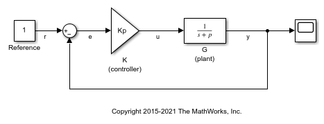
In this model:

Create an slLinearizer interface for the model.

sllin = slLinearizer(mdl);

To obtain the sensitivity at the plant input, u, add u as an analysis point to sllin.

addPoint(sllin,'u');

Obtain the sensitivity at the plant input, u.

sys = getSensitivity(sllin,'u');
tf(sys)

ans =
 
  From input "u" to output "u":
  s + 5
  -----
  s + 8
 
Continuous-time transfer function.

The software uses a linearization input, du, and linearization output u to compute sys.

sys is the transfer function from du to u, which is equal to .

Specify Temporary Loop Opening for Sensitivity Function Calculation

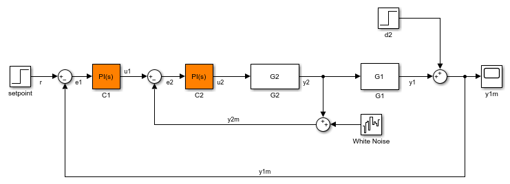
For the scdcascade model, obtain the inner-loop sensitivity at the output of G2, with the outer loop open.

Open the scdcascade model.

mdl = 'scdcascade';
open_system(mdl)

Create an slLinearizer interface for the model.

sllin = slLinearizer(mdl);

To calculate the sensitivity at the output of G2, use the y2 signal as the analysis point. To eliminate the effects of the outer loop, break the outer loop at y1m. Add both these points to sllin.

addPoint(sllin,{'y2','y1m'});

Obtain the sensitivity at y2 with the outer loop open.

sys = getSensitivity(sllin,'y2','y1m');

Here, 'y1m', the third input argument, specifies a temporary opening of the outer loop.

Obtain Sensitivity Function for Specific Parameter Combination

Suppose you batch linearize the scdcascade model for multiple transfer functions. For most linearizations, you vary the proportional (Kp2) and integral gain (Ki2) of the C2 controller in the 10% range. For this example, obtain the sensitivity at the output of G2, with the outer loop open, for the maximum values of Kp2 and Ki2.

Open the scdcascade model.

mdl = 'scdcascade';
open_system(mdl)

Create an slLinearizer interface for the model.

sllin = slLinearizer(mdl);

Vary the proportional (Kp2) and integral gain (Ki2) of the C2 controller in the 10% range.

Kp2_range = linspace(0.9*Kp2,1.1*Kp2,3);
Ki2_range = linspace(0.9*Ki2,1.1*Ki2,5);

[Kp2_grid,Ki2_grid] = ndgrid(Kp2_range,Ki2_range);

params(1).Name = 'Kp2';
params(1).Value = Kp2_grid;

params(2).Name = 'Ki2';
params(2).Value = Ki2_grid;

sllin.Parameters = params;

To calculate the sensitivity at the output of G2, use the y2 signal as the analysis point. To eliminate the effects of the outer loop, break the outer loop at y1m. Add both these points to sllin as analysis points.

addPoint(sllin,{'y2','y1m'});

Determine the index for the maximum values of Ki2 and Kp2.

mdl_index = params(1).Value == max(Kp2_range) & params(2).Value == max(Ki2_range);

Obtain the sensitivity at the output of G2 for the specified parameter combination.

sys = getSensitivity(sllin,'y2','y1m',mdl_index);

Obtain Offsets from Sensitivity Function

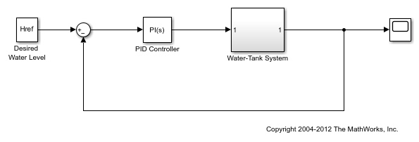
Open Simulink model.

mdl = 'watertank';
open_system(mdl)

Create a linearization option set, and set the StoreOffsets option.

opt = linearizeOptions('StoreOffsets',true);

Create slLinearizer interface.

sllin = slLinearizer(mdl,opt);

Add an analysis point at the tank output port.

addPoint(sllin,'watertank/Water-Tank System');

Calculate the sensitivity function at the analysis point, and obtain the corresponding linearization offsets.

[sys,info] = getSensitivity(sllin,'watertank/Water-Tank System');

View offsets.

info.Offsets

ans = 

  struct with fields:

             x: [2x1 double]
            dx: [2x1 double]
             u: 1
             y: 1
     StateName: {2x1 cell}
     InputName: {'watertank/Water-Tank System'}
    OutputName: {'watertank/Water-Tank System'}
            Ts: 0

Input Arguments

s — Interface to Simulink^® model

slLinearizer interface | slTuner interface

Interface to a Simulink model, specified as either an slLinearizer interface or an slTuner interface.

pt — Analysis point signal name

character vector | string | cell array of character vectors | string array

Analysis point signal name, specified as:

• Character vector or string — Analysis point signal name.

  To determine the signal name associated with an analysis point, type s. The software displays the contents of s in the MATLAB^® command window, including the analysis point signal names, block names, and port numbers. Suppose that an analysis point does not have a signal name, but only a block name and port number. You can specify pt as the block name. To use a point not in the list of analysis points for s, first add the point using addPoint.

  You can specify pt as a uniquely matching portion of the full signal name or block name. Suppose that the full signal name of an analysis point is 'LoadTorque'. You can specify pt as 'Torque' as long as 'Torque' is not a portion of the signal name for any other analysis point of s.

  For example, pt = 'y1m'.

• Cell array of character vectors or string array — Specifies multiple analysis point names. For example, pt = {'y1m','y2m'}.

To calculate linsys, the software adds a linearization input, followed by a linearization output at pt.

Consider the following model:

Specify pt as 'u':

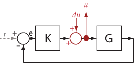
The software computes linsys as the transfer function from du to u.

If you specify pt as multiple signals, for example pt = {'u','y'}, the software adds a linearization input, followed by a linearization output at each point.

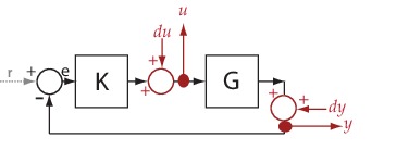
du and dy are linearization inputs, and, u and y are linearization outputs. The software computes linsys as a MIMO transfer function with a transfer function from each linearization input to each linearization output.

temp_opening — Temporary opening signal name

character vector | string | cell array of character vectors | string array

Temporary opening signal name, specified as:

• Character vector or string — Analysis point signal name.

  temp_opening must specify an analysis point that is in the list of analysis points for s. To determine the signal name associated with an analysis point, type s. The software displays the contents of s in the MATLAB command window, including the analysis point signal names, block names, and port numbers. Suppose that an analysis point does not have a signal name, but only a block name and port number. You can specify temp_opening as the block name. To use a point not in the list of analysis points for s, first add the point using addPoint.

  You can specify temp_opening as a uniquely matching portion of the full signal name or block name. Suppose that the full signal name of an analysis point is 'LoadTorque'. You can specify temp_opening as 'Torque' as long as 'Torque' is not a portion of the signal name for any other analysis point of s.

  For example, temp_opening = 'y1m'.

• Cell array of character vectors or string array — Specifies multiple analysis point names. For example, temp_opening = {'y1m','y2m'}.

mdl_index — Index for linearizations of interest

array of logical values | vector of positive integers

Index for linearizations of interest, specified as:

• Array of logical values — Logical array index of linearizations of interest. Suppose that you vary two parameters, par1 and par2, and want to extract the linearization for the combination of par1 > 0.5 and par2 <= 5. Use:

  params = s.Parameters;
  mdl_index = params(1).Value>0.5 & params(2).Value <= 5;

  The expression params(1).Value>0.5 & params(2).Value<5 uses logical indexing and returns a logical array. This logical array is the same size as params(1).Value and params(2).Value. Each entry contains the logical evaluation of the expression for corresponding entries in params(1).Value and params(2).Value.

• Vector of positive integers — Linear index of linearizations of interest. Suppose that you vary two parameters, par1 and par2, and want to extract the linearization for the combination of par1 > 0.5 and par2 <= 5. Use:

  params = s.Parameters;
  mdl_index = find(params(1).Value>0.5 & params(2).Value <= 5);

  The expression params(1).Value>0.5 & params(2).Value<5 returns a logical array. find returns the linear index of every true entry in the logical array

Output Arguments

linsys — Sensitivity function

state-space model

Sensitivity function, returned as described in the following:

• If you did not configure s.Parameters and s.OperatingPoints, the software calculates linsys using the default model parameter values. The software uses the model initial conditions as the linearization operating point. linsys is returned as a state-space model.

• If you configured s.Parameters only, the software computes a linearization for each parameter grid point. linsys is returned as a state-space model array of the same size as the parameter grid.

• If you configured s.OperatingPoints only, the software computes a linearization for each specified operating point. linsys is returned as a state-space model array of the same size as s.OperatingPoints.

• If you configured s.Parameters and specified s.OperatingPoints as a single operating point, the software computes a linearization for each parameter grid point. The software uses the specified operating point as the linearization operating point. linsys is returned as a state-space model array of the same size as the parameter grid.

• If you configured s.Parameters and specified s.OperatingPoints as multiple operating point objects, the software computes a linearization for each parameter grid point. The software requires that s.OperatingPoints is the same size as the parameter grid specified by s.Parameters. The software computes each linearization using corresponding operating points and parameter grid points. linsys is returned as a state-space model array of the same size as the parameter grid.

• If you configured s.Parameters and specified s.OperatingPoints as multiple simulation snapshot times, the software simulates and linearizes the model for each snapshot time and parameter grid point combination. Suppose that you specify a parameter grid of size p and N snapshot times. linsys is returned as a state-space model array of size N-by-p.

For most models, linsys is returned as an ss object or an array of ss objects. However, if your model contains one of the following blocks in the linearization path defined by pt, then linsys returns the specified type of state-space model.

Block	linsys Type
Block with a substitution specified as a genss object or tunable model object	genss
Block with a substitution specified as an uncertain model, such as uss	uss (Robust Control Toolbox)
Sparse Second Order block	mechss
Descriptor State-Space block configured to linearize to a sparse model	sparss

info — Linearization information

structure

Linearization information, returned as a structure with the following fields:

Offsets — Linearization offsets

[] (default) | structure | structure array

Linearization offsets, returned as [] if s.Options.StoreOffsets is false. Otherwise, Offsets is returned as one of the following:

• If linsys is a single state-space model, then Offsets is a structure.

• If linsys is an array of state-space models, then Offsets is a structure array with the same dimensions as linsys.

Each offset structure has the following fields:

Field	Description
x	State offsets used for linearization, returned as a column vector of length nx, where nx is the number of states in linsys.
y	Output offsets used for linearization, returned as a column vector of length ny, where ny is the number of outputs in linsys.
u	Input offsets used for linearization, returned as a column vector of length nu, where nu is the number of inputs in linsys.
dx	Derivative offsets for continuous time systems or updated state values for discrete-time systems, returned as a column vector of length nx.
StateName	State names, returned as a cell array that contains nx elements that match the names in linsys.StateName.
InputName	Input names, returned as a cell array that contains nu elements that match the names in linsys.InputName.
OutputName	Output names, returned as a cell array that contains ny elements that match the names in linsys.OutputName.
Ts	Sample time of the linearized system, returned as a scalar that matches the sample time in linsys.Ts. For continuous-time systems, Ts is 0.

If Offsets is a structure array, you can configure an LPV System block using the offsets. To do so, first convert them to the required format using getOffsetsForLPV. For an example, see Approximate Nonlinear Behavior Using Array of LTI Systems.

Advisor — Linearization diagnostic information

[] (default) | LinearizationAdvisor object | array of LinearizationAdvisor objects

Linearization diagnostic information, returned as [] if s.Options.StoreAdvisor is false. Otherwise, Advisor is returned as one of the following:

• If linsys is a single state-space model, Advisor is a LinearizationAdvisor object.

• If linsys is an array of state-space models, Advisor is an array of LinearizationAdvisor objects with the same dimensions as linsys.

LinearizationAdvisor objects store linearization diagnostic information for individual linearized blocks. For an example of troubleshooting linearization results using a LinearizationAdvisor object, see Troubleshoot Linearization Results at Command Line.

More About

Sensitivity Function

The sensitivity function, also referred to simply as sensitivity, measures how sensitive a signal is to an added disturbance. Sensitivity is a closed-loop measure. Feedback reduces the sensitivity in the frequency band where the open-loop gain is greater than 1.

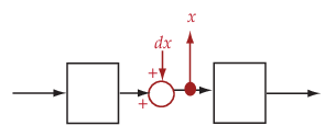
To compute the sensitivity at an analysis point, x, the software injects a disturbance signal, dx, at the point. Then, the software computes the transfer function from dx to x, which is equal to the sensitivity function at x.

Analysis Point in Simulink Model	How getSensitivity Interprets Analysis Point	Sensitivity Function
		Transfer function from dx to x

For example, consider the following model where you compute the sensitivity function at u:

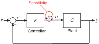
Here, the software injects a disturbance signal (du) at u. The sensitivity at u, Su, is the transfer function from du to u. The software calculates Su as follows:

$$\begin{array}{l}u=du-KGu\\ \to (I+KG)u=du\\ \to u={(}^{I}du\\ \therefore S_u={(}^I\end{array}$$

Here, I is an identity matrix of the same size as KG.

Similarly, to compute the sensitivity at y, the software injects a disturbance signal (dy) at y. The software computes the sensitivity function as the transfer function from dy to y. This transfer function is equal to (I+GK)^-1, where I is an identity matrix of the same size as GK.

The software does not modify the Simulink model when it computes the sensitivity transfer function.

Analysis Point

Analysis points, used by the slLinearizer and slTuner interfaces, identify locations within a model that are relevant for linear analysis and control system tuning. You use analysis points as inputs to the linearization commands, such as getIOTransfer, getLoopTransfer, getSensitivity, and getCompSensitivity. As inputs to the linearization commands, analysis points can specify any open-loop or closed-loop transfer function in a model. You can also use analysis points to specify design requirements when tuning control systems using commands such as systune.

Location refers to a specific block output port within a model or to a bus element in such an output port. For convenience, you can use the name of the signal that originates from this port to refer to an analysis point.

You can add analysis points to an slLinearizer or slTuner interface, s, when you create the interface. For example:

s = slLinearizer('scdcascade',{'u1','y1'});

Alternatively, you can use the addPoint command.

To view all the analysis points of s, type s at the command prompt to display the interface contents. For each analysis point of s, the display includes the block name and port number and the name of the signal that originates at this point. You can also programmatically obtain a list of all the analysis points using getPoints.

For more information about how you can use analysis points, see Mark Signals of Interest for Control System Analysis and Design and Mark Signals of Interest for Batch Linearization.

Permanent Openings

Permanent openings, used by the slLinearizer and slTuner interfaces, identify locations within a model where the software breaks the signal flow. The software enforces these openings for linearization and tuning. Use permanent openings to isolate a specific model component. Suppose that you have a large-scale model capturing aircraft dynamics and you want to perform linear analysis on the airframe only. You can use permanent openings to exclude all other components of the model. Another example is when you have cascaded loops within your model and you want to analyze a specific loop.

Location refers to a specific block output port within a model. For convenience, you can use the name of the signal that originates from this port to refer to an opening.

You can add permanent openings to an slLinearizer or slTuner interface, s, when you create the interface or by using the addOpening command. To remove a location from the list of permanent openings, use the removeOpening command.

To view all the openings of s, type s at the command prompt to display the interface contents. For each permanent opening of s, the display includes the block name and port number and the name of the signal that originates at this location. You can also programmatically obtain a list of all the permanent loop openings using getOpenings.

Version History

Introduced in R2013b

R2020b: Linearize Simulink model to a sparse state-space model

You can linearize and obtain a sparse model from a Simulink model that contains a Sparse Second Order or Descriptor State-Space block.

• mechss model when you use a Sparse Second Order in your Simulink model.

• sparss model when you use a Descriptor State-Space block and select the Linearize to sparse model block parameter.

For more information, see Sparse Model Basics. For an example, see Linearize Simulink Model to a Sparse Second-Order Model Object.

R2016b: Compute operating point offsets for model inputs, outputs, states, and state derivatives during linearization

You can compute operating point offsets for model inputs, outputs, states, and state derivatives when linearizing Simulink models. Thee offsets streamline the creation of linear parameter-varying (LPV) systems.

To obtain operating point offsets, first create a linearizeOptions or slTunerOptions object and set the StoreOffsets option to true. Then, create an slLinearizer or slTuner interface for the model.

You can extract the offsets from the info output argument of getSensitivity and convert them into the required format for the LPV System block using the getOffsetsForLPV function.