Main Content

umargin

Model gain and phase uncertainty

Since R2020a

Description

Use the umargin control design block to model gain and phase variations in feedback loops. Modeling gain and phase variations in your system lets you verify stability margins during robustness analysis or enforce them during robust controller design.

To add gain and phase uncertainty to a feedback loop, you incorporate umargin blocks into an uncertain state-space (uss) model of the closed-loop system. umargin is a SISO control design block, representing gain and phase variation at a single location in a single feedback loop. To model gain and phase uncertainty in MIMO feedback systems, insert a separate umargin object at each location in the system at which you want to introduce gain and phase uncertainty.

umargin models gain and phase variations as a factor F multiplying the open-loop response L. This factor takes values in a disk centered on the real axis and containing F = 1. You specify this disk by its intersection DGM = [gmin,gmax] with the real axis, which represents the relative amount of gain variation around the nominal value F = 1. To specify both gain and phase uncertainty, first use getDGM to obtain a DGM value that describes a disk that captures both your specified gain and phase ranges. For more information about the disk-based uncertainty model, see Algorithms.

When you have a uss model containing umargin control design blocks, you can perform robustness and worst-case analysis to examine how gain and phase variation affects the response of the system. For instance, use robstab and robgain to analyze the robust stability and robust performance of a system with gain and phase uncertainty. Use wcgain and wcsigmaplot to examine the worst-case responses of the system.

Requiring robust stability for a closed-loop system with umargin gain and phase uncertainty is equivalent to enforcing a disk-based gain margin [gmin,gmax] and corresponding phase margin. Therefore, you can use umargin blocks to enforce suitable disk margins when designing robust controllers with musyn.

Creation

Description

example

F = umargin(name,DGM) models relative gain uncertainty in the range DGM = [gmin,gmax] with gmin < 1 and gmax > 1. The gain modeled by F varies in this range for phase held at its nominal value. When you have both gain and phase uncertainty, use getDGM to find the corresponding DGM. This syntax also sets the Name property of F.

example

F = umargin(name,GM) is the same as umargin(name,[1/GM,GM]). This syntax specifies a gain that can increase or decrease by a factor GM in the absence of phase uncertainty. The corresponding amount of phase uncertainty is determined by the disk-based uncertainty model that umargin uses (see Algorithms).

F = umargin(___,Name,Value) sets additional properties of F using name-value pairs. For example, F = umargin('F',[0.8,1.4],'InputName','u0','OutputName','u') creates a umargin block and sets the input and output names for use with connect. Enclose each property name in quotes.

Input Arguments

expand all

Range of relative gain variation, specified as a two-element vector of the form [gmin,gmax], where gmin < 1 and gmax > 1. For instance, DGM = [0.8 1.5] means that the modeled gain can vary between 80% and 150% of its nominal value (that is, change by a factor between 0.8 and 1.5). gmin can be negative, defining a range of relative gain variation that includes a change in sign.

The modeled uncertainty includes the corresponding phase variation determined by the disk-based uncertainty model (see Algorithms). To get the gain range DGM that best represents the gain and phase variation that you want to model, use getDGM.

Amount of gain increase or decrease, specified as a scalar. For instance, if you use GM = 2, then the umargin block represents a gain that can increase or decrease by a factor of two. umargin(name,GM) is equivalent to umargin(name,[1/GM,GM]). The resulting modeled uncertainty includes the corresponding phase variation determined by the disk-based uncertainty model (see Algorithms).

Properties

expand all

Range of relative gain variation in absolute units, specified as a two-element vector of the form gmin, gmax, where gmin < 1 and gmax > 1. For example GainChange = [0.8,1.5] means that the gain can vary between 80% and 150% of its nominal value. gmin can be negative, which models possible sign changes in the loop gain.

The relationship between this property and the PhaseChange, DiskMargin, and Skew properties is determined by the disk-based uncertainty model that umargin uses (see Algorithms). If you change the value of this property on an existing umargin block, the other properties are automatically updated.

This property is read-only.

Amount of phase variation in degrees, specified as two-element vector of the form [-pm,pm]. The value of this property is determined by the value of GainChange and the disk-based uncertainty model that umargin uses (see Algorithms).

Example: [-30,30]

Normalized uncertainty level, specified as a positive scalar. This value is the parameter ɑ that sets the size of the uncertainty disk (see Algorithms).

The relationship between this property and the GainChange, PhaseChange, and Skew properties is determined by the disk-based uncertainty model that umargin uses. If you change the value of this property on an existing umargin block, the other properties are automatically updated.

Example: 0.5

Skew of the modeled uncertainty disk, specified as a scalar value. The skew biases the modeled gain variation toward gain increase or decrease.

  • Skew = 0 models a balanced gain range [gmin,gmax], with gmin = 1/gmax.

  • Positive Skew models a varying gain that can increase more than it can decrease, gmax > 1/gmin). For instance, GainChange = [0.8,2] corresponds to a positive Skew value, because the gain can increase by 100% but decrease by only 20%.

  • Negative Skew models a varying gain that can decrease more than it can increase, gmin < 1/gmax. For instance, GainChange = [0.5,1.2] corresponds to a negative Skew value, because the can decrease by 50% but increase by only 20%.

The larger the absolute value of Skew, the more the gain range is biased. For additional details about Skew and how it affects the disk-based uncertainty model, see Stability Analysis Using Disk Margins.

The relationship between this property and the GainChange, PhaseChange, and DiskMargin properties is determined by the disk-based uncertainty model that umargin uses (see Algorithms). If you change the value of this property on an existing umargin block, the other properties are automatically updated.

Number of states in random samples of the block, specified as an integer. Some analysis commands such as usample and bode take random samples of uncertain dynamics. This property determines the number of states in the samples. For more information about how sampling of dynamic uncertainty works, see Generate Samples of Uncertain Systems.

Maximum frequency of random samples, specified as a positive scalar value. Randomly sampled uncertain dynamics are no faster than the specified value.

This property is read-only.

Nominal value, specified as a state-space model representing a SISO static gain of 1 (A, B, C = 0, D = 1). The nominal value of a umargin block is always 1 (no gain and phase variation) regardless of the range of gain and phase variations the block represents.

Block simplification level, specified as 'basic', 'full', or 'off'. In general, when you combine uncertain elements to create uncertain state-space models, the software automatically applies techniques to eliminate redundant copies of the uncertain elements. (See simplify.) Use this property to specify the simplification to apply when you use model arithmetic or interconnection techniques with the uncertain block.

  • 'basic' — Apply the elementary simplification method after each arithmetical or interconnection operation.

  • 'full' — Apply techniques similar to model reduction.

  • 'off' — Perform no simplification.

Name of uncertain element, specified as a character vector. When you create an uncertain state-space (uss or genss) model using uncertain control design blocks, the software tracks the blocks using the name you specify in this property, not the variable name in the MATLAB® workspace. For example, if you create a umargin block using F = umargin('um',2), and combine the block with a numeric LTI model, the Blocks property of the resulting uss model lists the uncertain control design block um.

Sample time, specified as:

  • 0 — For continuous-time models.

  • Positive scalar value — For discrete-time models. Specify the sample time in the units given in the TimeUnit property of the model.

  • –1 — For discrete-time models with unspecified sample time.

Changing this property does not discretize or resample the model.

Model time units, specified as:

  • 'nanoseconds'

  • 'microseconds'

  • 'milliseconds'

  • 'seconds'

  • 'minutes'

  • 'hours'

  • 'days'

  • 'weeks'

  • 'months'

  • 'years'

If you specify TimeUnit using a string, such as "hours", the time units are stored as a character vector, 'hours'.

Model properties such as sample time Ts, InputDelay, OutputDelay, and other time delays are expressed in the units specified by TimeUnit. Changing this property has no effect on other properties, and therefore changes the overall system behavior. Use to convert between time units without modifying system behavior.

Name of input channel, specified as a cell array containing a character vector. You can set InputName using a character vector, such as F.InputName = 'u', or using a string, such as F.InputName = "u". Either way, the input name is stored as a cell array containing a character vector, {'u'}.

Units of input signal, specified as a cell array containing a character vector. Use InputUnit to keep track of the units each input signal is expressed in. InputUnit has no effect on system behavior. You can set InputUnit using a character vector, such as F.InputUnit = 'V', or using a string, such as F.InputUnit = "V". Either way, the input name is stored as a cell array containing a character vector, {'V'}.

Input channel groups, specified as a structure where the fields are the group names and the values are the indices of the input channels belonging to the corresponding group. Because umargin blocks are always SISO, you do not need to specify input groups.

Name of output channel, specified as a cell array containing a character vector. You can set OutputName using a character vector, such as F.OutputName = 'y', or using a string, such as F.OutputName = "y". Either way, the output name is stored as a cell array containing a character vector, {'y'}.

Units of output signal, specified as a cell array containing a character vector. Use OutputUnit to keep track of the units each output signal is expressed in. OutputUnit has no effect on system behavior. You can set OutputUnit using a character vector, such as F.OutputUnit = 'V', or using a string, such as F.OutputUnit = "V". Either way, the output name is stored as a cell array containing a character vector, {'V'}.

Output channel groups, specified as a structure where the fields are the group names and the values are the indices of the input channels belonging to the corresponding group. Because umargin blocks are always SISO, you do not need to specify output groups.

Text notes about the model, specified as a string or character vector. The property stores whichever of these two data types you provide. For instance, suppose that sys1 and sys2 are dynamic system models. You can set their Notes properties to a string and a character vector, respectively.

sys1.Notes = "sys1 has a string.";
sys2.Notes = 'sys2 has a character vector.';
sys1.Notes
sys2.Notes
ans = 

    "sys1 has a string."


ans =

    'sys2 has a character vector.'

You can also specify Notes as string array or a cell array of character vectors or strings.

Data of any kind that you want to associate and store with the model, specified as any MATLAB data type.

Object Functions

Many functions that work on numeric LTI models also work on uncertain control design blocks such as umargin. These include model interconnection functions such as connect and feedback, and linear analysis functions such as bode and stepinfo. Some functions that generate plots, such as bode and step, plot random samples of the uncertain model to give you a sense of the distribution of uncertain dynamics. When you use these commands to return data, however, they operate on the nominal value of the system only. The following lists contain a representative subset of the functions you can use with umargin models.

expand all

feedbackFeedback connection of multiple models
connectBlock diagram interconnections of dynamic systems
seriesSeries connection of two models
parallelParallel connection of two models
uscaleScale uncertainty of block or system
plot (umargin)Visualize gain and phase uncertainty of a umargin block
usampleGenerate random samples of uncertain model or element
usubsSubstitute given values for uncertain elements of uncertain objects
stepStep response of dynamic system
bodeBode plot of frequency response, or magnitude and phase data

Examples

collapse all

Create a model of a SISO control loop, with gain uncertainty of ±6 dB and phase uncertainty of ±30°. Use open-loop transfer function

L=3.5s3+2s2+3s.

L = tf(2.5,[1 2 3 0]);

To model the uncertainty, first use getDGM to convert the gain and phase variation into a disk-based gain-margin range. Because the gain can increase or decrease by the same amount, you can use the 'balanced' option to model a disk of uncertainty that is symmetric around the nominal value.

GM = db2mag(6);
PM = 30;
DGM = getDGM(GM,PM,'balanced')
DGM = 1×2

    0.5012    1.9953

DGM defines a disk of uncertainty with gain variations in the range given by DGM, and phase variations determined by the geometry of the disk. Use DGM to create a umargin block.

F = umargin('F',DGM)
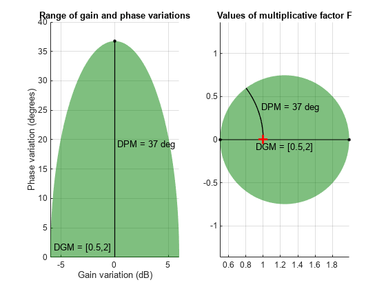
Uncertain gain/phase "F" with relative gain change in [0.501,2] and phase change of ±36.8 degrees.

F represents the smallest uncertainty disk that can capture both the target gain and phase variation. The actual phase variation modeled by F is a little bigger than the target range of ±30°. To visualize the full range of gain and phase variations represented by F, including simultaneous gain and phase variations, use plot.

plot(F)

The right plot shows the range of values in the complex plane that the multiplicative factor F can take. The size of the disk determines the amount of variation. The shaded region on the left plot shows the simultaneous variations of gain and phase encompassed in F. For more details about this uncertainty model, see Stability Analysis Using Disk Margins.

To incorporate the gain and phase uncertainty into a model of the closed-loop system, insert it into the feedback loop as a multiplicative factor on the open-loop response.

T = feedback(L*F,1)
Uncertain continuous-time state-space model with 1 outputs, 1 inputs, 3 states.
The model uncertainty consists of the following blocks:
  F: Uncertain gain/phase, gain × [0.501,2], phase ± 36.8 deg, 1 occurrences

Type "T.NominalValue" to see the nominal value and "T.Uncertainty" to interact with the uncertain elements.

The result is an uncertain state-space (uss) model with one control design block, F. Examine the effect of the modeled gain and phase uncertainty on the step response of the closed-loop system.

figure;
rng default  % for reproducibility
step(T)

You can perform addition analysis with this model, such as analyzing the system robustness against the modeled gain and phase variation with robstab. Or, you can use musyn to design a robust controller for the uncertain system L*F. For examples, see

Create a umargin block that models gain that can decrease by 10% but increase by 60% in the absence of phase variation, and a phase variation of ±15° in the absence of gain variation. To do so, use getDGM with the 'tight' option. This option finds the smallest disk that captures the gain and phase ranges you provide.

DGM = getDGM([0.9,1.6],[-15,15],'tight');
F = umargin('F',DGM)
Uncertain gain/phase "F" with relative gain change in [0.86,1.6] and phase change of ±15 degrees.

In this case, the smallest disk encompasses the specified phase variation, and a gain variation that is slightly larger, but still skews toward increases in gain. Visualize the corresponding disk and the ranges of gain and phase variations modeled by F.

plot(F)

The left-hand plot shows that the modeled gain variation is not symmetric around the nominal value.

Generate another umargin block, this time using the 'balanced' option in getDGM.

DGMb = getDGM([0.9,1.6],[-15,15],'balanced');
Fb = umargin('Fb',DGMb);

Compare the uncertainty disk modeled by each block.

figure;
diskmarginplot([F.GainChange;Fb.GainChange],'disk')

The disk of Fb models a larger, symmetric gain range (gmin = 1/gmax) and larger phase variations than the ones you specify. If you are confident that gain varies more in one direction than the other in your system, then this balanced model might be overly conservative.

The umargin block represents a SISO gain and phase uncertainty. To model gain and phase variations in a MIMO feedback loop, create a umargin block for each location in the loop at which you want to introduce gain and phase variation. For instance, consider the two-input, two-output feedback loop of the example MIMO Stability Margins for Spinning Satellite.

Suppose that you want to study the system's behavior with gain and phase variations at the plant inputs and outputs. You can model those variations by creating separate umargin blocks for each channel, and building them into the closed-loop model.

Create the plant and controller models from MIMO Stability Margins for Spinning Satellite. The plant is a two-input, two-output state-space model, and the feed-forward filter Kf is a two-input, two-output static gain.

% Plant
a = 10;
A = [0 a;-a 0];
B = eye(2);
C = [1 a;-a 1];
D = 0;
P = ss(A,B,C,D);

% Prefilter
Kf = [1 -a;a 1]/(1+a^2);

Next, create the umargin blocks to represent the gain and phase uncertainty in each channel. Suppose that you want to model a gain uncertainty of about 5% in either direction at all four locations. Create a umargin block to model this uncertainty.

GM = 1.05;
u1 = umargin('u1',GM)
Uncertain gain/phase "u1" with relative gain change in [0.952,1.05] and phase change of ±2.79 degrees.

umargin converts the specified gain variation of ±5% to a disk-based uncertainty model, which also allows phase changes of about ±3°. Use plot to visualize the disk and the modeled range of gain and phase variation at each input and output.

plot(u1)

To get the best estimates of the impact of gain and phase uncertainty on system performance, you want the gain and phase to vary independently at each of the four locations. Therefore, create additional umargin blocks for each plant input and output, with the same gain specification.

u2 = umargin('u2',GM);
y1 = umargin('y1',GM);
y2 = umargin('y2',GM);

Build the closed-loop model, inserting u1 and u2 at the plant inputs, and y1 and y2 at the plant outputs. To do this, use blkdiag to combine u1 and u2 into a two-input, two-output system of the form [u1,0;0,u2]. Create a similar combination of y1 and y2. Then connect these with the plant, and use the feedback command to close the two-channel feedback loop.

Fu = blkdiag(u1,u2);
Fy = blkdiag(y1,y2);
L = Fy*P*Fu;    
Tunc = feedback(L,eye(2))*Kf
Uncertain continuous-time state-space model with 2 outputs, 2 inputs, 2 states.
The model uncertainty consists of the following blocks:
  u1: Uncertain gain/phase, gain × [0.952,1.05], phase ± 2.79 deg, 1 occurrences
  u2: Uncertain gain/phase, gain × [0.952,1.05], phase ± 2.79 deg, 1 occurrences
  y1: Uncertain gain/phase, gain × [0.952,1.05], phase ± 2.79 deg, 1 occurrences
  y2: Uncertain gain/phase, gain × [0.952,1.05], phase ± 2.79 deg, 1 occurrences

Type "Tunc.NominalValue" to see the nominal value and "Tunc.Uncertainty" to interact with the uncertain elements.

Examine the effect of these variations on the system response.

rng(1)  % for reproducibility
figure
step(Tunc,Tunc.NominalValue,10)

These small uncertainties have a considerable impact on system performance, sometimes even changing the sign of the response. Robustness analysis with robstab shows that only a slightly larger variation drives the closed-loop system unstable.

stabmarg = robstab(Tunc)
stabmarg = struct with fields:
           LowerBound: 1.0210
           UpperBound: 1.0231
    CriticalFrequency: 1.0000e-04

The requirement that a closed-loop system is robust against a particular amount of gain and phase uncertainty is equivalent to saying that the system has that amount of gain and phase margin. You can therefore use a umargin block to check the gain and phase margins of a system that also requires robustness against other types of uncertainty. To do so, capture your required disk margins in a umargin block, and use robstab to check robust stability against all uncertainty modeled in the system.

Consider the following closed-loop system with parameter uncertainty.

k = ureal('k',10,'Percent',40);
G = tf(18,[1 k k]);
C = pid(1,2);
CL = feedback(G*C,1);

robstab shows that the system is robust against the modeled uncertainty. In fact, the system remains stable up two a little more than twice the modeled uncertainty.

stabmarg = robstab(CL)
stabmarg = struct with fields:
           LowerBound: 2.0458
           UpperBound: 2.0458
    CriticalFrequency: 4.4517

Suppose that you also require the system to tolerate gain increase or decrease of up to 50% and phase variation of up to ±20° at the plant input. To check whether the system has these margins, create a umargin block that models these variations and insert it into the closed-loop model.

DGM = getDGM(1.5,20,'tight');
F = umargin('F');
Gf = G*F;
CLf = feedback(Gf*C,1);

stabmarg = robstab(CLf)
stabmarg = struct with fields:
           LowerBound: 1.0933
           UpperBound: 1.0957
    CriticalFrequency: 3.9553

This result shows that in addition to robust stability against parameter variation, the feedback loop also maintains the desired gain and phase margins for all modeled values of k (actually for about 9% more than the modeled range of k).

You can also use the equivalence between disk margins and robust stability to gain and phase variations to design a robust controller that satisfies certain gain and phase margins. For examples, see Design Robust Controller With Specified Gain and Phase Margins and Robust Controller for Spinning Satellite.

The robust controller returned by musyn optimizes robust performance of uncertain feedback systems. When the uncertain plant contains umargin blocks, this requirement of robust stability is equivalent to enforcing disk-based gain and phase margins equal to the umargin uncertainty. In this example, design a robust controller for an uncertain plant, enforcing closed-loop stability against gain and phase variations at the plant inputs and outputs.

Use the plant from the example "Loop Shaping with mixsyn" on the mixsyn reference page, introducing some uncertainty in the location of the system poles and zero.

a = ureal('a',1,'PlusMinus',[-0.1,0.1]);
s = zpk('s');
G = (s-a)/(s+a)^2;

The goal is to enforce closed-loop stability against gain and phase variation at the plant inputs and outputs, over the full range of parameter variation modeled in the plant G. To do so, use the target gain and phase margins to create umargin uncertain blocks and attach them to the plant. For this example, suppose that you want stability against gain variations of a factor of 1.5 in either direction, or phase variations of ±20°.

DGM = getDGM(1.5,20,'tight');
Fin = umargin('Fin',DGM);
Fout = umargin('Fout',DGM);
Gmarg = Fout*G*Fin
Uncertain continuous-time state-space model with 1 outputs, 1 inputs, 7 states.
The model uncertainty consists of the following blocks:
  Fin: Uncertain gain/phase, gain × [0.667,1.5], phase ± 22.6 deg, 1 occurrences
  Fout: Uncertain gain/phase, gain × [0.667,1.5], phase ± 22.6 deg, 1 occurrences
  a: Uncertain real, nominal = 1, variability = [-0.1,0.1], 3 occurrences

Type "Gmarg.NominalValue" to see the nominal value and "Gmarg.Uncertainty" to interact with the uncertain elements.

For tuning with musyn, you augment the plant with weighting functions that enforce your performance requirement such as reference tracking, disturbance rejection, and robustness. For this example, use the weighting functions described in the example on the on the mixsyn reference page.

W1 = makeweight(10,[1 0.1],0.01);
W2 = makeweight(0.1,[32 0.32],1);
W3 = makeweight(0.01,[1 0.1],10);

Gaug = augw(Gmarg,W1,W2,W3);

Use musyn to design a controller.

[K,gam] = musyn(Gaug,1,1);
D-K ITERATION SUMMARY:
-----------------------------------------------------------------
                       Robust performance               Fit order
-----------------------------------------------------------------
  Iter         K Step       Peak MU       D Fit             D
    1           7.753        1.527        1.539            24
    2           1.131        1.084        1.091            40
    3               1       0.9963        1.003            38
    4          0.9968       0.9942        1.002            40
    5          0.9984       0.9928       0.9989            42

Best achieved robust performance: 0.993

musyn achieves a robust performance of about 1, which tells you that the closed-loop gain remains below 1 for the full range of uncertainty specified in the plant. To confirm that the resulting controller achieves the target gain and phase margins, use wcdiskmargin to examine the worst-case gain and phase margins of the system against simultaneous variations at the plant inputs and outputs. Use the plant G that contains the parameter uncertainty but not the gain and phase uncertainty.

MMIO = wcdiskmargin(G,K)
MMIO = struct with fields:
           GainMargin: [0.6027 1.6591]
          PhaseMargin: [-27.8421 27.8421]
           DiskMargin: 0.4957
           LowerBound: 0.4957
           UpperBound: 0.4967
    CriticalFrequency: 0.9228
    WorstPerturbation: [1x1 struct]

The worst-case disk-based gain margin of [0.6 1.66] is slightly larger than the target margin of [0.66 1.5], and the worst-case phase margin of ±28° is likewise better than the required margin of ±20°. Thus, the controller K enforces the desired margins for the entire parameter-uncertainty range of the plant G.

For an example that uses umargin blocks with musyn to enforce gain and phase margins in a MIMO control loop, see Robust Controller for Spinning Satellite.

Consider a umargin block that captures a gain variation of a factor of 1.5 in either direction, and a phase variation of ±20°.

DGM = getDGM(1.5,20,'tight');
F = umargin('F',DGM)
Uncertain gain/phase "F" with relative gain change in [0.667,1.5] and phase change of ±22.6 degrees.

When you create the umargin object, you provide the target disk-based gain variation DGM, which defines a disk of uncertainty. This value becomes the property F.GainChange, and umargin sets other properties based on this value. For instance, F.PhaseChange is automatically set to the phase range corresponding to the uncertainty disk defined by DGM. The properties F.DiskMargin and F.Skew are automatically set to the corresponding α and σ values of the disk (see Algorithms). Examine the values of these properties.

get(F)
              GainChange: [0.6667 1.5000]
             PhaseChange: [-22.6199 22.6199]
              DiskMargin: 0.4000
                    Skew: 0
    SampleStateDimension: 3
      SampleMaxFrequency: Inf
            NominalValue: [1x1 ss]
            AutoSimplify: 'basic'
                    Name: 'F'
               InputName: {''}
               InputUnit: {''}
              InputGroup: [1x1 struct]
              OutputName: {''}
              OutputUnit: {''}
             OutputGroup: [1x1 struct]
                   Notes: [0x1 string]
                UserData: []
                      Ts: 0
                TimeUnit: 'seconds'

You can change the amount of modeled gain and phase uncertainty using the uscale command, which scales the normalized uncertainty of the block by a factor you specify. Scale the uncertainty of F by one half, and examine the properties of the scaled uncertain block.

Fscaled = uscale(F,0.5)
Uncertain gain/phase "F" with relative gain change in [0.818,1.22] and phase change of ±11.4 degrees.
get(Fscaled)
              GainChange: [0.8182 1.2222]
             PhaseChange: [-11.4212 11.4212]
              DiskMargin: 0.2000
                    Skew: 0
    SampleStateDimension: 3
      SampleMaxFrequency: Inf
            NominalValue: [1x1 ss]
            AutoSimplify: 'basic'
                    Name: 'F'
               InputName: {''}
               InputUnit: {''}
              InputGroup: [1x1 struct]
              OutputName: {''}
              OutputUnit: {''}
             OutputGroup: [1x1 struct]
                   Notes: [0x1 string]
                UserData: []
                      Ts: 0
                TimeUnit: 'seconds'

For umargin blocks, uscale multiplies the DiskMargin property by the scaling factor, scaling the size of the disk and adjusting the ranges of gain and phase variations accordingly.

If you manually change any of the properties that relate to the size of the modeled uncertainty, the block automatically updates the values of all of them. For instance, set F.GainChange to a new value that defines a different uncertainty disk. The properties of F are automatically updated to reflect the new corresponding phase range (F.PhaseChange) and the values of α and σ (F.DiskMargin and F.Skew) that describe the new disk.

F.GainChange = [0.8,1.5];
get(F)
              GainChange: [0.8000 1.5000]
             PhaseChange: [-16.9574 16.9574]
              DiskMargin: 0.2857
                    Skew: 2.0000
    SampleStateDimension: 3
      SampleMaxFrequency: Inf
            NominalValue: [1x1 ss]
            AutoSimplify: 'basic'
                    Name: 'F'
               InputName: {''}
               InputUnit: {''}
              InputGroup: [1x1 struct]
              OutputName: {''}
              OutputUnit: {''}
             OutputGroup: [1x1 struct]
                   Notes: [0x1 string]
                UserData: []
                      Ts: 0
                TimeUnit: 'seconds'

Here, F.PhaseChange, F.DiskMargin, and F.Skew are all updated to describe the disk defined by the new value of F.GainChange. The new value of F.Skew is non-zero, because the new gain range is not symmetric (gmin1/gmax).

Algorithms

umargin models gain and phase variations in an individual feedback channel as a frequency-dependent multiplicative factor F(s) multiplying the nominal open-loop response L(s), such that the perturbed response is L(s)F(s). The factor F(s) is parameterized by:

F(s)=1+α[(1σ)/2]δ(s)1α[(1+σ)/2]δ(s).

In this model,

  • δ(s) is a gain-bounded dynamic uncertainty, normalized so that it always varies within the unit disk (||δ|| < 1).

  • ɑ sets the amount of gain and phase variation modeled by F. For fixed σ, the parameter ɑ controls the size of the disk. For ɑ = 0, the multiplicative factor is 1, corresponding to the nominal L.

  • σ, called the skew, biases the modeled uncertainty toward gain increase or gain decrease.

The factor F takes values in a disk centered on the real axis and containing the nominal value F = 1. The disk is characterized by its intercept DGM = [gmin,gmax] with the real axis. gmin < 1 and gmin > 1 are the minimum and maximum relative changes in gain modeled by F, at nominal phase. The phase uncertainty modeled by F is the range DPM = [pmin,pmax] of phase values at the nominal gain (|F| = 1). For instance, in the following plot, the right side shows the disk F that intersects the real axis in the interval [0.71,1.4]. The left side shows that this disk models a gain variation of ±3 dB and a phase variation of ±19°.

F = umargin('F',1.4125)
plot(F)

Multiplicative disk and range of gain and phase variations for umargin block modeling gain variation of plus or minus 3 dB and phase variation of plus or minus 19 degrees.

When you create a umargin block, you specify the amount of uncertainty by specifying DGM. Use getDGM to translate specific amounts of gain and phase variations in to a suitable DGM range that captures these variations. For more information about the uncertainty model used by umargin, see Stability Analysis Using Disk Margins.
Version History

Introduced in R2020a

expand all