pdeplot
Plot solution or mesh for 2-D problem
Syntax
Description
pdeplot(results.Mesh,XYData=results.Temperature,ColorMap="hot")
plots the temperature at nodal locations for a 2-D thermal analysis problem.
This syntax creates a colored surface plot using the "hot"
colormap.
pdeplot(results.Mesh,XYData=results.VonMisesStress,Deformation=results.Displacement)
plots the von Mises stress and shows the deformed shape for a 2-D structural
analysis problem.
pdeplot(results.Mesh,XYData=results.ModeShapes.ux) plots
the x-component of the modal displacement for a 2-D
structural modal analysis problem.
pdeplot(results.Mesh,XYData=results.ElectricPotential)
plots the electric potential at nodal locations for a 2-D electrostatic analysis
problem.
pdeplot(results.Mesh,XYData=results.NodalSolution) plots
the solution at nodal locations as a colored surface plot using the default
colormap.
pdeplot( plots the mesh
specified in model)model. This syntax does not work with an
femodel object.
pdeplot(___,
plots the mesh, the data at the nodal locations, or both the mesh and the data,
using the Name,Value)Name,Value pair arguments. Use any arguments from
the previous syntaxes.
Specify at least one of the FlowData (vector field plot),
XYData (colored surface plot), or
ZData (3-D height plot) name-value pairs. You can
combine any number of plot types.
For a thermal analysis, you can plot temperature or gradient of temperature.
For a structural analysis, you can plot displacement, stress, strain, and von Mises stress. In addition, you can show the deformed shape and specify the scaling factor for the deformation plot.
For an electromagnetic analysis, you can plot electric or magnetic potentials, fields, and flux densities.
Examples
Solve a 2-D transient thermal problem.
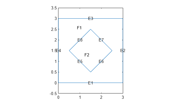
Create a geometry representing a square plate with a diamond-shaped region in its center.
SQ1 = [3; 4; 0; 3; 3; 0; 0; 0; 3; 3];
D1 = [2; 4; 0.5; 1.5; 2.5; 1.5; 1.5; 0.5; 1.5; 2.5];
gd = [SQ1 D1];
sf = 'SQ1+D1';
ns = char('SQ1','D1');
ns = ns';
g = decsg(gd,sf,ns);
pdegplot(g,EdgeLabels="on",FaceLabels="on")
xlim([-1.5 4.5])
ylim([-0.5 3.5])
axis equal
Create an femodel object for transient thermal analysis and include the geometry.
model = femodel(AnalysisType="thermalTransient", ...
                Geometry=g);
For the square region, assign these thermal properties:
Thermal conductivity is
Mass density is
Specific heat is
model.MaterialProperties(1) = ...
    materialProperties(ThermalConductivity=10, ...
                       MassDensity=2, ...
                       SpecificHeat=0.1);
For the diamond region, assign these thermal properties:
Thermal conductivity is
Mass density is
Specific heat is
model.MaterialProperties(2) = ...
    materialProperties(ThermalConductivity=2, ...
                       MassDensity=1, ...
                       SpecificHeat=0.1);
Assume that the diamond-shaped region is a heat source with a density of .
model.FaceLoad(2) = faceLoad(Heat=4);
Apply a constant temperature of 0 °C to the sides of the square plate.
model.EdgeBC(1:4) = edgeBC(Temperature=0);
Set the initial temperature to 0 °C.
model.FaceIC = faceIC(Temperature=0);
Generate the mesh.
model = generateMesh(model);
The dynamics for this problem are very fast. The temperature reaches a steady state in about 0.1 second. To capture the most active part of the dynamics, set the solution time to logspace(-2,-1,10). This command returns 10 logarithmically spaced solution times between 0.01 and 0.1.
tlist = logspace(-2,-1,10);
Solve the equation.
thermalresults = solve(model,tlist);
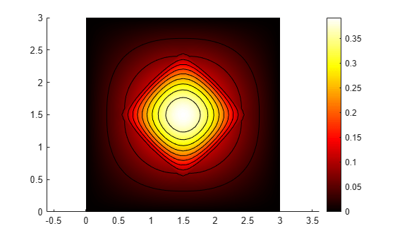
Plot the solution with isothermal lines by using a contour plot.
T = thermalresults.Temperature;
msh = thermalresults.Mesh;
pdeplot(msh,XYData=T(:,10),Contour="on",ColorMap="hot")
axis equal
Create an femodel object for structural analysis and include the unit square geometry in the model.
model = femodel(AnalysisType="structuralStatic", ...
                Geometry=@squareg);
Plot the geometry.
pdegplot(model.Geometry,EdgeLabels="on")
xlim([-1.1 1.1])
ylim([-1.1 1.1])
Specify Young's modulus and Poisson's ratio.
model.MaterialProperties = ...
    materialProperties(PoissonsRatio=0.3, ...
                       YoungsModulus=210E3);
Specify the x-component of the enforced displacement for edge 1.
model.EdgeBC(1) = edgeBC(XDisplacement=0.001);
Specify that edge 3 is a fixed boundary.
model.EdgeBC(3) = edgeBC(Constraint="fixed");Generate a mesh and solve the problem.
model = generateMesh(model);
R = solve(model);
Plot the deformed shape using the default scale factor. By default, pdeplot internally determines the scale factor based on the dimensions of the geometry and the magnitude of deformation.
pdeplot(R.Mesh, ...
        XYData=R.VonMisesStress, ...
        Deformation=R.Displacement, ...
        ColorMap="jet")
axis equal

Plot the deformed shape with the scale factor 500.
pdeplot(R.Mesh, ...
        XYData=R.VonMisesStress, ...
        Deformation=R.Displacement, ...
        DeformationScaleFactor=500,...
        ColorMap="jet")
axis equal

Plot the deformed shape without scaling.
pdeplot(R.Mesh, ...
        XYData=R.VonMisesStress, ...
        ColorMap="jet")
axis equal

Find the fundamental (lowest) mode of a 2-D cantilevered beam, assuming prevalence of the plane-stress condition.
Specify geometric and structural properties of the beam, along with a unit plane-stress thickness.
length = 5;
height = 0.1;
E = 3E7;
nu = 0.3;
rho = 0.3/386;
Create a geometry.
gdm = [3;4;0;length;length;0;0;0;height;height];
g = decsg(gdm,'S1',('S1')');
Create an femodel object for modal structural analysis and include the geometry.
model = femodel(Analysistype="structuralModal", ...
                Geometry=g);
Define a maximum element size (five elements through the beam thickness).
hmax = height/5;
Generate a mesh.
model=generateMesh(model,Hmax=hmax);
Specify the structural properties and boundary constraints.
model.MaterialProperties = ...
    materialProperties(YoungsModulus=E, ...
                       MassDensity=rho, ...
                       PoissonsRatio=nu);
model.EdgeBC(4) = edgeBC(Constraint="fixed");
Compute the analytical fundamental frequency (Hz) using the beam theory.
I = height^3/12;
analyticalOmega1 = 3.516*sqrt(E*I/(length^4*(rho*height)))/(2*pi)
analyticalOmega1 =
126.9498
Specify a frequency range that includes an analytically computed frequency and solve the model.
R = solve(model,FrequencyRange=[0,1e6])
R =
  ModalStructuralResults with properties:

    NaturalFrequencies: [32×1 double]
            ModeShapes: [1×1 FEStruct]
                  Mesh: [1×1 FEMesh]
The solver finds natural frequencies and modal displacement values at nodal locations. To access these values, use R.NaturalFrequencies and R.ModeShapes.
R.NaturalFrequencies/(2*pi)
ans = 32×1
105 ×

    0.0013
    0.0079
    0.0222
    0.0433
    0.0711
    0.0983
    0.1055
    0.1462
    0.1930
    0.2455
    0.2948
    0.3034
    0.3664
    0.4342
    0.4913
      ⋮
R.ModeShapes
ans =
  FEStruct with properties:

           ux: [6511×32 double]
           uy: [6511×32 double]
    Magnitude: [6511×32 double]
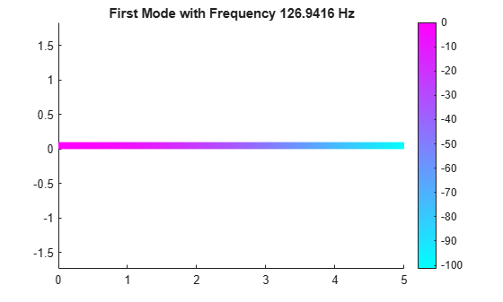
Plot the y-component of the solution for the fundamental frequency.
pdeplot(R.Mesh,XYData=R.ModeShapes.uy(:,1))
title(['First Mode with Frequency ', ...
        num2str(R.NaturalFrequencies(1)/(2*pi)),' Hz'])
axis equal
Solve an electromagnetic problem and find the electric potential and field distribution for a 2-D geometry representing a plate with a hole.
Create an femodel object for electrostatic analysis and include a geometry representing a plate with a hole.
model = femodel(AnalysisType="electrostatic",...
                Geometry="PlateHolePlanar.stl");
Plot the geometry with edge labels.
pdegplot(model.Geometry,EdgeLabels="on")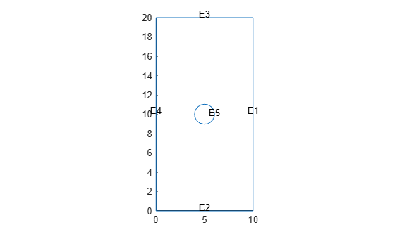
Specify the vacuum permittivity value in the SI system of units.
model.VacuumPermittivity = 8.8541878128E-12;
Specify the relative permittivity of the material.
model.MaterialProperties = ...
    materialProperties(RelativePermittivity=1);
Apply the voltage boundary conditions on the edges framing the rectangle and the circle.
model.EdgeBC(1:4) = edgeBC(Voltage=0);
model.EdgeBC(5) = edgeBC(Voltage=1000);
Specify the charge density for the entire geometry.
model.FaceLoad = faceLoad(ChargeDensity=5E-9);
Generate the mesh.
model = generateMesh(model);
Solve the model.
R = solve(model)
R =
  ElectrostaticResults with properties:

      ElectricPotential: [1231×1 double]
          ElectricField: [1×1 FEStruct]
    ElectricFluxDensity: [1×1 FEStruct]
                   Mesh: [1×1 FEMesh]
Plot the electric potential distribution using the Contour parameter to display equipotential lines and the Levels parameter to specify how many equipotential lines to display.
pdeplot(R.Mesh,XYData=R.ElectricPotential, ...
               Contour="on", ...
               Levels=5)
axis equal
You can also use the Levels parameter to specify electric potential values for which to display equipotential lines.
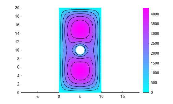
pdeplot(R.Mesh,XYData=R.ElectricPotential, ...
               Contour="on", ...
               Levels=[500 1500 2500 4000])
axis equal

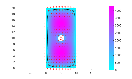
Now plot the electric potential, the equipotential line for the potential value 750, and a quiver plot representing the electric field.
pdeplot(R.Mesh,XYData=R.ElectricPotential, ...
               Contour="on", ...
               Levels=[750 750], ...
               FlowData=[R.ElectricField.Ex ...
                         R.ElectricField.Ey])
axis equal
Create colored 2-D and 3-D plots of a solution to a PDE model.
Create a PDE model. Include the geometry of the built-in function lshapeg. Mesh the geometry.
model = createpde;
geometryFromEdges(model,@lshapeg);
generateMesh(model);
Set the zero Dirichlet boundary conditions on all edges.
applyBoundaryCondition(model,"dirichlet", ...
                             Edge=1:model.Geometry.NumEdges, ...
                             u=0);
Specify the coefficients and solve the PDE.
specifyCoefficients(model,m=0, ...
                          d=0, ...
                          c=1, ...
                          a=0, ...
                          f=1);
results = solvepde(model)
results =
  StationaryResults with properties:

    NodalSolution: [1141×1 double]
       XGradients: [1141×1 double]
       YGradients: [1141×1 double]
       ZGradients: []
             Mesh: [1×1 FEMesh]
Plot the 2-D solution at the nodal locations.
u = results.NodalSolution;
msh = results.Mesh;
pdeplot(msh,XYData=u)
axis equal
Plot the 3-D solution.
pdeplot(msh,XYData=u,ZData=u)

Plot the gradient of a PDE solution as a quiver plot.
Create a PDE model. Include the geometry of the built-in function lshapeg. Mesh the geometry.
model = createpde;
geometryFromEdges(model,@lshapeg);
generateMesh(model);
Set the zero Dirichlet boundary conditions on all edges.
applyBoundaryCondition(model,"dirichlet", ...
                             Edge=1:model.Geometry.NumEdges, ...
                             u=0);
Specify coefficients and solve the PDE.
specifyCoefficients(model,m=0, ...
                          d=0, ...
                          c=1, ...
                          a=0, ...
                          f=1);
results = solvepde(model)
results =
  StationaryResults with properties:

    NodalSolution: [1141×1 double]
       XGradients: [1141×1 double]
       YGradients: [1141×1 double]
       ZGradients: []
             Mesh: [1×1 FEMesh]
Plot the gradient of the solution at the nodal locations as a quiver plot.
ux = results.XGradients;
uy = results.YGradients;
msh = results.Mesh;
pdeplot(msh,FlowData=[ux,uy])
axis equal
Plot the solution of a 2-D PDE in 3-D with the "jet" coloring and a mesh, and include a quiver plot. Get handles to the axes objects.
Create a PDE model. Include the geometry of the built-in function lshapeg. Mesh the geometry.
model = createpde;
geometryFromEdges(model,@lshapeg);
generateMesh(model);
Set zero Dirichlet boundary conditions on all edges.
applyBoundaryCondition(model,"dirichlet", ...
                             Edge=1:model.Geometry.NumEdges, ...
                             u=0);
Specify coefficients and solve the PDE.
specifyCoefficients(model,m=0, ...
                          d=0, ...
                          c=1, ...
                          a=0, ...
                          f=1);
results = solvepde(model)
results =
  StationaryResults with properties:

    NodalSolution: [1141×1 double]
       XGradients: [1141×1 double]
       YGradients: [1141×1 double]
       ZGradients: []
             Mesh: [1×1 FEMesh]
Plot the solution in 3-D with the "jet" coloring and a mesh, and include the gradient as a quiver plot.
u = results.NodalSolution;
ux = results.XGradients;
uy = results.YGradients;
msh = results.Mesh;
h = pdeplot(msh,XYData=u,ZData=u, ...
                FaceAlpha=0.5, ...
                FlowData=[ux,uy], ...
                ColorMap="jet", ...
                Mesh="on");

Since R2026a
Position two Axes objects in a figure. Add the solution plot to one object and the geometry plot to another object.
Solve a heat transfer problem on the unit square geometry.
model = femodel(AnalysisType="thermalSteady", ...
    Geometry=@squareg);
model.MaterialProperties = ...
    materialProperties(ThermalConductivity=1);
model.EdgeBC(3) = edgeBC(Temperature=100);
model.EdgeLoad(1) = edgeLoad(Heat=-10);
model = generateMesh(model);
results = solve(model);
Specify the position of the first Axes object so that it has a lower left corner at the point (0.1 0.1) with a width and height of 0.7. Specify the position of the second Axes object so that it has a lower left corner at the point (0.4 0.65) with a width and height of 0.3. By default, the values are normalized to the figure. Return the Axes objects as ax1 and ax2.
ax1 = axes(Position=[0.1 0.1 0.7 0.7]);
ax2 = axes(Position=[0.4 0.65 0.3 0.3]);
Plot the temperature distribution and the geometry adding the temperature distribution plot to ax1 and the geometry plot to ax2.
pdeplot(ax1,results.Mesh,XYData=results.Temperature)
pdegplot(ax2,model.Geometry,EdgeLabels="on")
xlim(ax2,[-1.2 1.2])
ylim(ax2,[-1.2 1.2])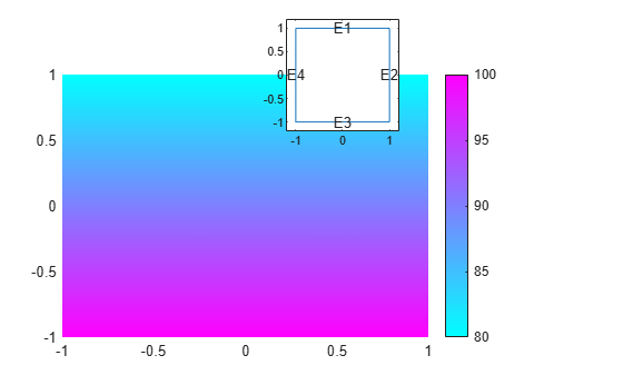
Create an femodel object and include the geometry of the built-in function lshapeg.
model = femodel(Geometry=@lshapeg);
Generate and plot the mesh.
model = generateMesh(model,Hmax=0.3, ...
                     GeometricOrder="linear");
msh = model.Geometry.Mesh;
pdeplot(msh)

Alternatively, you can use the nodes and elements of the mesh as input arguments for pdeplot.
pdeplot(msh.Nodes,msh.Elements)

Display the node labels.
pdeplot(msh,NodeLabels="on")
Display the element labels.
pdeplot(msh,ElementLabels="on")