Detect Attack in Cyber-Physical Systems Using Dynamic Watermarking
Cyber-physical systems (CPS) consist of communication channels that transmit data between the sensors and actuators in the physical plants and the controller. These channels are susceptible to faults and attacks that disrupt or degrade the operation and can even lead to catastrophic failures in such closed-loop systems.

This example demonstrates the detection of such attacks in a networked DC microgrid system using dynamic watermarking [1]. The technique adds an excitation (watermark) to the secure controller command and detects attacks by monitoring the observed signals for distortions of the watermark.
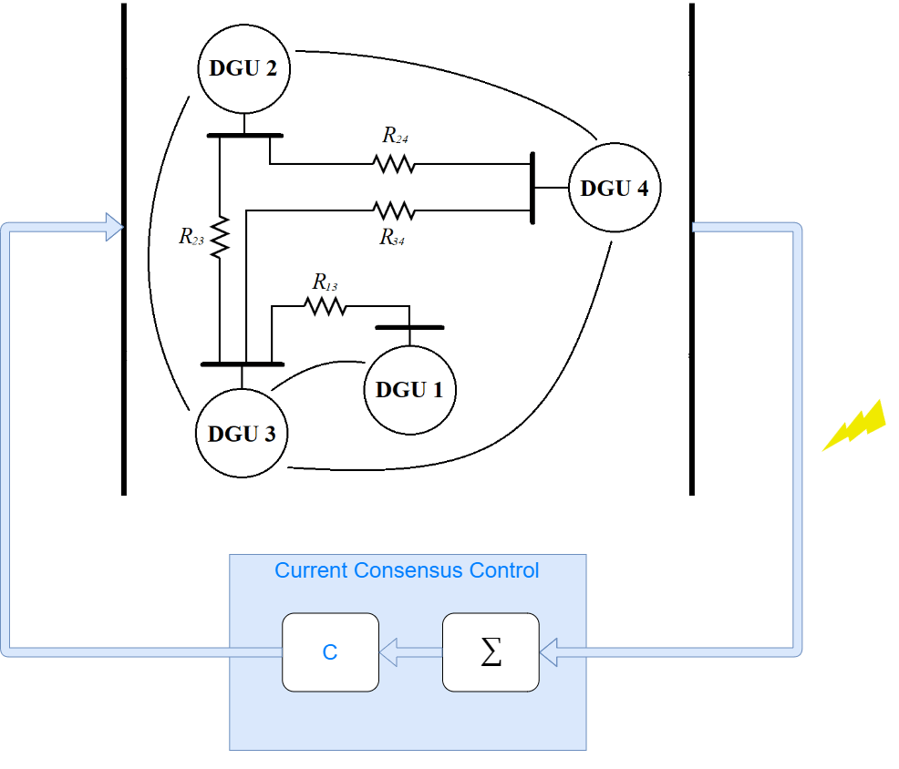
DC Microgrid Model with Current Consensus Control
Distributed generation units (DGU) in a DC microgrid (DCmG) represent physical nodes in a networked CPS. The central controller adjusts the reference voltages in each DGU to share current loads equally across multiple units.
See Detect Replay Attacks in DC Microgrids Using Distributed Watermarking for more details on the plant model and controller parameters.
Use a sample time of 50 microseconds and a simulation duration of 3 seconds.
Ts = 5e-5;
Vin = 100;
Ct = 2.2e-3;
Lt = 1.8e-3;
Rt = 0.2;

Lij = 1.8e-6;
Rij = 0.05;

Vref = 48;
Kp = 0.1;
Ki = 6.15;
Kd = 4.6e-4;
N = 2.56e3;
Tf = 1/N;
The current controller is designed to share the load current in the individual nodes and maintain the ratio of the individual line capacities. Define the capacity of the first DGU to be twice of the other three nodes.
K = 150;
Icapacity = [2 1 1 1];

M = ones(4,4);
M(1,1) = -1/Icapacity(1);
M(1,[2 3 4]) = 1/sum(Icapacity([2 3 4]));
M(2,2) = -1/Icapacity(2);
M(2,[1 3 4]) = 1/sum(Icapacity([1 3 4]));
M(3,3) = -1/Icapacity(3);
M(3,[1 2 4]) = 1/sum(Icapacity([1 2 4]));
M(4,4) = -1/Icapacity(4);
M(4,[1 2 3]) = 1/sum(Icapacity([1 2 3]));
The load current is applied using Controlled Current Source blocks and is modified at different instances to see the effect on all nodes.
ILoadInitial = [5, 5, 5, 5];
ILoadChanged = [2, 4, 1.5, 3];
tLoadChanged = [0.5, 0.75, 1.0, 1.25];
Simulate Model in Nominal Condition
Set the variables that enable (true) or disable (false) the watermarking, attack, and attack detection subsystems.
enableWatermark = false;
enableAttack = false;
enableAttackDetection = false;
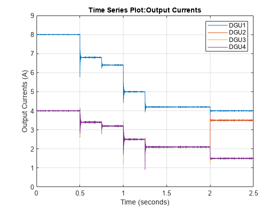
Simulate the model to see the effect of load changes. You can observe that the line currents of the different DGUs maintain the ratio of their capacities with every load change.
modelName = 'DynamicWatermarkingInDCMicroGrid';
open_system(modelName);

simInput = Simulink.SimulationInput(modelName);
out = sim(simInput);

figure;
plot(out.DGU_LineCurrents);
ylim([0 9]);
grid on
legend('DGU1','DGU2','DGU3','DGU3');

Linearize Model
The monitoring strategy uses the plant model for detecting changes in the closed-loop signals. Use linearize (Simulink Control Design) to obtain a linear approximation of the DCmG at a steady-state operating point.
You can use findop (Simulink Control Design) to get snapshot operating point after system is at steady-state, at t = 0.3 seconds. The local sample-based solver in the Solver Configuration block is disabled to support linearization operations.
op = findop(modelName,0.3);
Define the input to the plant as the output of the controller, and the load current inputs that are needed to prevent false detections of load disturbance changes as attacks or faults. The outputs of the plant are the line currents of each DGU.
io(1) = linio([modelName,'/Current Consensus Controller'],1,'openinput');
io(2) = linio([modelName,'/DC Microgrid/ILoad_1'],1,'openinput');
io(3) = linio([modelName,'/DC Microgrid/ILoad_2'],1,'openinput');
io(4) = linio([modelName,'/DC Microgrid/ILoad_3'],1,'openinput');
io(5) = linio([modelName,'/DC Microgrid/ILoad_4'],1,'openinput');
io(6) = linio([modelName,'/Select line currents'],1,'openoutput');
Linearize the plants based on the defined analysis and operating points. Store the offsets information for use in the attack detection strategy.
opts = linearizeOptions(StoreOffsets=true,SampleTime=Ts);
[linsys,~,info] = linearize(modelName,io,op,opts);
Dynamic Watermarking
This model adds a random excitation signal, , drawn from a Gaussian distribution with zero mean, to the voltage command that the controller to each physical node communicates. Since the controller is secure, this signal is not known to the external agents. You must model the power of the excitation signal carefully based on voltage levels such that it does not modify the desired operation of the closed-loop control. However, it should be high enough to differentiate between attacks and disturbance due to noise.

The sensor measurements are correlated with the known, secure watermark, with signal power . Statistical tests are used to develop conditions that should be satisfied in when sensors are reporting the true output. Any distortion in the signals would result in the computed sequence of measurements cross the threshold indicating an attack.
Let the states of the multiple input, multiple output plant be represented by the following state-space model.
where represents the controller command and is the injected watermark.
As shown in [1], the statistical tests are then defined as follows.
is generated for the ith actuator, and represents the ith column of .
For partially observed systems, such as the DCmG used in this example, use a Kalman Filter block with the linearized model linsys to estimate the state vector. The offset information stored in info is subtracted from the input and output measurements before being used to generate the estimated states and the statistical test outputs and .

enableWatermark = true;
watermarkVariance = [1e-6, 1e-6, 1e-6, 1e-6];
Attack Detection
The communication channel is attacked at t = 2 seconds and the line current measurements are modified to change the balance of the DGUs in the networked cyber-physical system. The model settings is configured to start at steady state.
The detection tests and generate signals of dimensions -by- and -by-1, respectively, where is the order of the linearized plant system. Signals at specific indices, defined in detectionTest1_StateIndex and detectionTest2_StateIndex, are extracted and plotted to observe the detection response when an attack occurs.
enableAttack = true;
tAttack = 2;
IAttack = [1 0 -1 0 1 0 1 0];

enableAttackDetection = true;
actuatorIndex = 1;
detectionTest1_StateIndex = [1 1];
detectionTest2_StateIndex = 1;

simInput = setModelParameter(simInput,'LoadExternalInput','on');
simInput = setModelParameter(simInput,'ExternalInput','getinputstruct(op)');
simInput = setModelParameter(simInput,'LoadInitialState','on');
simInput = setModelParameter(simInput,'InitialState','getstatestruct(op)');

out = sim(simInput);
As seen in the output current plot below, the output of DGU 2 increases at the expense of other units when the system is attacked.
figure;
plot(out.DGU_LineCurrents);
grid on;
legend('DGU1','DGU2','DGU3','DGU4');
The detection tests generate two sequences. The first element of each sequence is extracted and shown below. Both tests indicate an attack after t = 2 seconds when it does not satisfy the condition based on the plant model.
figure;
plot(out.AttackDetectionTest1);
grid on
figure;
plot(out.AttackDetectionTest2);
grid on
References
[1] B. Satchidanandan and P. R. Kumar, "Dynamic Watermarking: Active Defense of Networked Cyber–Physical Systems," in Proceedings of the IEEE, vol. 105, no. 2, pp. 219-240, Feb. 2017, doi: 10.1109/JPROC.2016.2575064.
See Also
Average-Value DC-DC
Converter (Simscape Electrical) | Kalman Filter | linearize (Simulink Control Design)