Ergebnisse für
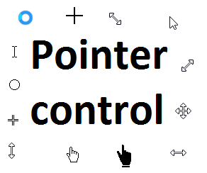
Starting in r2020a , you can change the mouse pointer symbol in apps and uifigures.
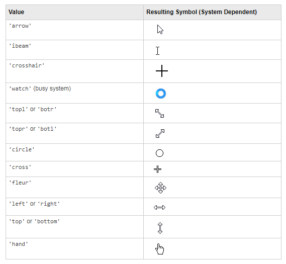
The Pointer property of a figure defines the cursor’s default pointer symbol within the figure. You can also create your own pointer symbols (see part 3, below).
Part 1. How to define a default pointer symbol for a uifigure or app
For figures or uifigures, set the pointer property when you define the figure or change the pointer property using the figure handle.
% Set pointer when creating the figure
uifig = uifigure('Pointer', 'crosshair');
% Change pointer after creating the figure
uifig.Pointer = 'crosshair';
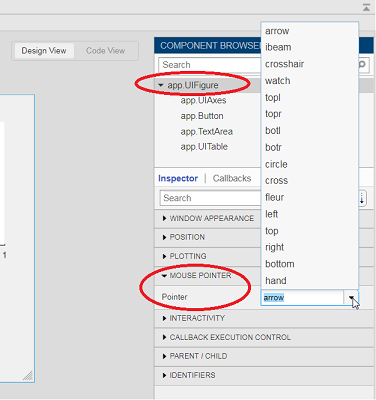
For apps made in AppDesigner, you can either set the pointer from the Design View or you can set the pointer property of the app’s UIFigure from the startup function using the second syntax shown above.
Part 2. How to change the pointer symbol dynamically
The pointer can be changed by setting specific conditions that trigger a change in the pointer symbol.
For example, the pointer can be temporarily changed to a busy-symbol when a button is pressed. This ButtonPushed callback function changes the pointer for 1 second.
function WaitasecondButtonPushed(app, event)
   % Change pointer for 1 second.
   set(app.UIFigure, 'Pointer','watch')
   pause(1)
   % Change back to default.
   set(app.UIFigure, 'Pointer','arrow')
   app.WaitasecondButton.Value = false;
end
The pointer can be changed every time it enters or leaves a uiaxes or any plotted object within the uiaxes. This is controlled by a set of pointer management functions that can be set in the app’s startup function.
iptSetPointerBehavior(obj,pointerBehavior) allows you to define what happens when the pointer enters, leaves, or moves within an object. Currently, only axes and axes objects seem to be supported for UIFigures.
iptPointerManager(hFigure,'enable') enables the figure’s pointer manager and updates it to recognize the newly added pointer behaviors.
The snippet below can be placed in the app’s startup function to change the pointer to crosshairs when the pointer enters the outerposition of a uiaxes and then change it back to the default arrow when it leaves the uiaxes.
% Define pointer behavior when pointer enter axes
pm.enterFcn = @(~,~) set(app.UIFigure, 'Pointer', 'crosshair');
pm.exitFcn  = @(~,~) set(app.UIFigure, 'Pointer', 'arrow');
pm.traverseFcn = [];
iptSetPointerBehavior(app.UIAxes, pm)
% Enable pointer manager for app
iptPointerManager(app.UIFigure,'enable');
Any function can be triggered when entering/exiting an axes object which makes the pointer management tools quite powerful. This snippet below defines a custom function cursorPositionFeedback() that responds to the pointer entering/exiting a patch object plotted within the uiaxes. When the pointer enters the patch, the patch color is changed to red, the pointer is changed to double arrows, and text appears in the app’s text area. When the pointer exits, the patch color changes back to blue, the pointer changes back to crosshairs, and the text area is cleared.
% Plot patch on uiaxes
hold(app.UIAxes, 'on')
region1 = patch(app.UIAxes,[1.5 3.5 3.5 1.5],[0 0 5 5],'b','FaceAlpha',0.07,...
    'LineWidth',2,'LineStyle','--','tag','region1');
% Define pointer behavior for patch
pm.enterFcn = @(~,~) cursorPositionFeedback(app, region1, 'in');
pm.exitFcn  = @(~,~) cursorPositionFeedback(app, region1, 'out');
pm.traverseFcn = [];
iptSetPointerBehavior(region1, pm)
% Enable pointer manager for app
iptPointerManager(app.UIFigure,'enable');
function cursorPositionFeedback(app, hobj, inout)
% When inout is 'in', change hobj facecolor to red and update textbox.
% When inout is 'out' change hobj facecolor to blue, and clear textbox.
% Check tag property of hobj to identify the object.
switch lower(inout)
    case 'in'
        facecolor = 'r';
        txt = 'Inside region 1';
        pointer = 'fleur';
    case 'out'
        facecolor = 'b';
        txt = '';
        pointer = 'crosshair';
end
hobj.FaceColor = facecolor;
app.TextArea.Value = txt;
set(app.UIFigure, 'Pointer', pointer)
end
The app showing the demo below is attached.
Part 3. Create your own custom pointer symbol
- Set the figure’s pointer property to ‘custom’.
- Set the figure’s PointerShapeCData property to the custom pointer matrix. A custom pointer is defined by a 16x16 or 32x32 matrix where NaN values are transparent, 1=black, and 2=white.
- Set the figure’s PointerShapeHotSpot to [m,n] where m and n are the coordinates that define the tip or "hotspot" of the matrix.
This demo uses the attached mat file to create a black hand pointer symbol.
iconData = load('blackHandPointer.mat');
uifig = uifigure();
uifig.Pointer = 'custom';
uifig.PointerShapeCData = iconData.blackHandIcon;
uifig.PointerShapeHotSpot = iconData.hotspot;
Also see Jiro's pointereditor() function on the file exchange which allows you to draw your own pointer.
Starting in r2020a, AppDesigner buttons and TreeNodes can display animated GIFs, SVG, and truecolor image arrays.
Every component in the App above is either a Button or a TreeNode!
Prior to r2020a the icon property of buttons and TreeNodes in AppDesigner supported JPEG, PNG, or GIF image files specified by a character vector or string array but did not support animation.
Here's how to display an animated GIF, SVG, or truecolor image in an App button or TreeNode starting in r2020a. And for the record, "GIF" is pronounced with a hard-g .
Display an animated GIF
Select the button or TreeNode from within AppDesigner > Design View and navigate to Component Browser > Inspector > Button dropdown list of properties (shown below). Select an animated GIF file and set the text and icon alignment properties.
To set the icon property programmatically,
app.Button.Icon = 'launch.gif'; % or "launch.gif"
The filename can be an image file on the Matlab path (see addpath ) or a full path to an image file.
Display SVG
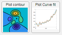
Use “scalable vector graphics” files for high-resolution images that are scaled to different sizes while preserving their shape and retaining their clarity. A quick and easy way to remember which plotting function is assigned to each button in an app is to assign an image of the plot to the button.
After creating the figure, expand the axes by setting the position or outerposition property to [0 0 1 1] in normalized units and save the figure using File > Save as and select svg format. Save the image to the folder containing your app. Then follow the same procedure as animated GIFs.
Display truecolor image
A truecolor image comes in the form of an [m x n x 3] array where each m x n pixel color is specified by an RGB triplet (read more) . This feature allows you to dynamically create a digital image or to upload an image from a mat file rather than an image file.
In this example, a progress bar is created within the uibutton callback function and it’s updated within a loop. For a complete demo of this feature see this comment .
% Button pushed function: ProcessDataButton
function ProcessDataButtonPushed(app, event)
    % Change button name to "Processing"
    app.ProcessDataButton.Text = 'Processing...';
    % Put text on top of icon
    app.ProcessDataButton.IconAlignment = 'bottom';
    % Create waitbar with same color as button
    wbar = permute(repmat(app.ProcessDataButton.BackgroundColor,15,1,200),[1,3,2]);
    % Black frame around waitbar
    wbar([1,end],:,:) = 0;
    wbar(:,[1,end],:) = 0;
    % Load the empty waitbar to the button
    app.ProcessDataButton.Icon = wbar;
    % Loop through something and update waitbar
    n = 10;
    for i = 1:n
        % Update image data (royalblue)
        % if mod(i,10)==0 % update every 10 cycles; improves efficiency
         currentProg = min(round((size(wbar,2)-2)*(i/n)),size(wbar,2)-2);
         RGB = app.ProcessDataButton.Icon;
         RGB(2:end-1, 2:currentProg+1, 1) = 0.25391; % (royalblue)
         RGB(2:end-1, 2:currentProg+1, 2) = 0.41016;
         RGB(2:end-1, 2:currentProg+1, 3) = 0.87891;
           app.ProcessDataButton.Icon = RGB;
          % Pause to slow down animation
          pause(.3)
          % end
      end
      % remove waitbar
      app.ProcessDataButton.Icon = '';
      % Change button name
      app.ProcessDataButton.Text = 'Process Data';
  end
The for-loop above was improved on Feb-11-2022.
Credit for the black & teal GIF icons: lordicon.com
New to r2020a, leapseconds() creates a table showing all leap seconds recognized by the datetime data type.
>> leapseconds()
ans =
  27×2 timetable
       Date        Type    CumulativeAdjustment
    ___________    ____    ____________________
    30-Jun-1972     +              1 sec
    31-Dec-1972     +              2 sec
    31-Dec-1973     +              3 sec
    31-Dec-1974     +              4 sec
    31-Dec-1975     +              5 sec
             << 21 rows removed >>
    31-Dec-2016     +             27 sec
Leap seconds can covertly sneak into your data and cause errors that are difficult to resolve if the leap seconds go undetected. A leap second was responsible for crashing Reddit , Mozilla, Yelp, LinkedIn and other sites in 2012.
Detect leap seconds present in a vector of years
% Define a vector of years
t = 2005:2008;
allLeapSeconds = leapseconds();
isYearWithLeapSecond = ismember(t,year(allLeapSeconds.Date));
% Show years that contain a leap second
t(isYearWithLeapSecond)
ans =
        2005        2008
Detect leap seconds present in a vector of months
% Define a vector of months
t = datetime(1972, 1, 1) + calmonths(0:11);
t.Format = 'MMM-yyyy';
allLeapSeconds = leapseconds();
[tY,tM] = ymd(t);
[leapSecY, leapSecM] = ymd(allLeapSeconds.Date);
isMonthWithLeapSecond = ismember([tY(:),tM(:)], [leapSecY, leapSecM], 'rows');
% Show months that contain a leap second
t(isMonthWithLeapSecond)
ans =
  1×2 datetime array
   Jun-1972   Dec-1972
List all leap seconds in your lifetime
% Enter your birthday in mm/dd/yyyy hh:mm:ss format
yourBirthday = '01/15/1988 14:30:00';
yourTimeRange = timerange(datetime(yourBirthday), datetime('now'));
allLeapSeconds = leapseconds();
lifeLeapSeconds = allLeapSeconds(yourTimeRange,:);
lifeLeapSeconds.YourAge = lifeLeapSeconds.Date - datetime(yourBirthday);
lifeLeapSeconds.YourAge.Format = 'y';
% Show table
fprintf('\n Leap seconds in your lifetime:\n')
disp(lifeLeapSeconds)
Leap seconds in your lifetime:
       Date        Type    CumulativeAdjustment     YourAge
    ___________    ____    ____________________    __________
    31-Dec-1989     +             15 sec           1.9587 yrs
    31-Dec-1990     +             16 sec            2.958 yrs
                        << 8 rows removed >>
    30-Jun-2012     +             25 sec           24.456 yrs
    30-Jun-2015     +             26 sec           27.454 yrs
    31-Dec-2016     +             27 sec            28.96 yrs
What is a leap second?
A second is defined as the time it takes a cesium-133 atom to oscillate 9,192,631,770 times under controlled conditions. The transition frequency is so precise that it takes 100 million years to gain 1 second of error [1]. If the earth’s rotation were perfectly synchronized to the atomic second, a day would be 86,400 seconds. But the earth’s rate of rotation is affected by climate, winds, atmospheric pressure, and the rate of rotation is gradually decreasing due to tidal friction [2,3]. Several months before the expected difference between the atomic clock-based time (UTC) and universal time (UT1) reaches +/- 0.9 seconds the IERS authorizes the addition (or subtraction) of 1 leap second (see plot below). Since the first leap second in 1972, all leap second adjustments have been made on the last day of June or December and all adjustments have been +1 second which explains the + signs in the type column of the leapseconds() table.
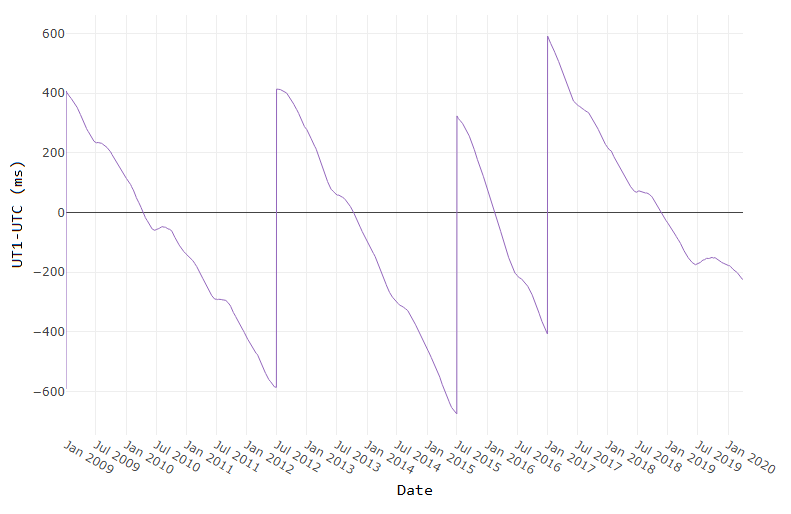
[ Image source ]
How to reference the leap second schedule in your code
Since leap second adjustments are not regularly timed, you can record the official IERS Bulletin C version used at the time of your analysis by accessing the 2nd output to leapseconds().
[T,vers] = leapseconds
What do leap seconds look like in datetime values?
A minute typically has 60 seconds spanning from 0:59. A minute containing a leap second has 61 seconds spanning from 0:60.
December 30, 2016 was a normal day. If we add the usual 86400 seconds to the start of that day, the result is the start of the next day.
d = datetime(2016, 12, 30, 'TimeZone','UTCLeapSeconds') + seconds(86400)
d =
  datetime
   2016-12-31T00:00:00.000Z
The next day, December 31, 2016, had a leap second. If we add 86400 seconds to the start of that day, the result is not the start of the next day.
d = datetime(2016, 12, 31, 'TimeZone','UTCLeapSeconds') + seconds(86400)
d =
  datetime
   2016-12-31T23:59:60.000Z
When will the next leap second be?
As of the current date (April 2020) the timing of the next leap second is unknown. Based on the data from the plot above, what's your guess?
References
Do date ranges from two different timetables intersect?
Is a specific datetime value within the range of a timetable?
Is the range of row times in a timetable within the limits of a datetime array?
Three new functions in r2020a will help to answer these questions.
- [tf, whichRows] = containsrange(TT,__)
- [tf, whichRows] = overlapsrange(TT,__)
- [tf, whichRows] = withinrange(TT,__)
In these function inputs, TT is a timetable and input #2 is one of the following:
- another timetable
- a time range object produced by timerange(startTime,endTime)
- a datetime scalar produced by datetime()
- a duration
The tf output is a logical scalar indicating pass|fail and the whichRows output is a logical vector identifying the rows of TT that are within the specified time range.
How do these functions differ?
Let's test all 3 functions with different time ranges and a timetable of electric utility outages in the United States, provided by Matlab. The first few rows of outages.csv are shown below in a timetable. You can see that the row times are not sorted which won't affect the behavior of these functions.
8×5 timetable
     OutageTime          Region         Loss     Customers     RestorationTime            Cause
  ________________    _____________    ______    __________    ________________    ___________________
  2002-02-01 12:18    {'SouthWest'}    458.98    1.8202e+06    2002-02-07 16:50    {'winter storm'   }
  2003-01-23 00:49    {'SouthEast'}    530.14    2.1204e+05                 NaT    {'winter storm'   }
  2003-02-07 21:15    {'SouthEast'}     289.4    1.4294e+05    2003-02-17 08:14    {'winter storm'   }
  2004-04-06 05:44    {'West'     }    434.81    3.4037e+05    2004-04-06 06:10    {'equipment fault'}
  2002-03-16 06:18    {'MidWest'  }    186.44    2.1275e+05    2002-03-18 23:23    {'severe storm'   }
  2003-06-18 02:49    {'West'     }         0             0    2003-06-18 10:54    {'attack'         }
  2004-06-20 14:39    {'West'     }    231.29           NaN    2004-06-20 19:16    {'equipment fault'}
  2002-06-06 19:28    {'West'     }    311.86           NaN    2002-06-07 00:51    {'equipment fault'}
The range of times in utility.csv is depicted by the gray timeline bar in the plot below labeled "Timetable row times". The timeline bars above it are various time ranges or scalar datetime values used to test the three new functions.
The three columns of checkboxes on the right of the plot show the results of the first output of each function, tf, for each time range.
The time ranges were created by the timerange function using the syntax timerange(startTime,endTime). The default intervalType in timerange() is 'openright' which means that datetimes are matched when they are equal to or greater than startTime and less than but not equal to endTime. The scalar datetime values were created with datetime().
The colorbar along with the colored points at the bottom of each timeline bar show the row numbers of timetable TT that were selected by the whichRows output of the three functions.
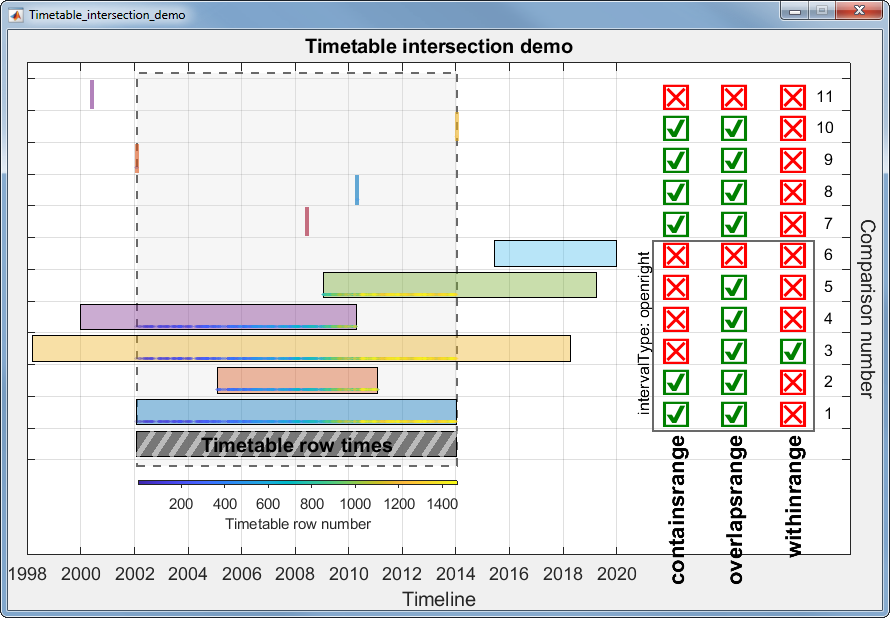
The containsrange() function returns true when all of the time range values are within the timetable including the timetable's minimum and maximum datetime.
The overlapsrange() function returns true when any of the time range values are with the timetable's range.
The withinrange() function returns true only when all of the timetable's datetime values are within the time range values. A careful observer may see that comparison number 1 is false even though that time range is exactly equal to the timetable's row time range. This is because the default value for intervalType in the timerange() function is 'openright' which does not match the end values if they are equal. If you change the intervalType to 'closed' the withinrange result for comparison 1 would be true.
The scalar datetime values for comparisons 8, 9 and 10 are all exact matches of datetimes within the timetable and result in a single match in the whichRows output. The datetime values for comparisons 7 and 11 do not match any of the timetable row times and the values in whichRows are all false even though comparison 7 is within the timetable range. For all three tests, the whichRows outputs are identical.
---------------------------------------------------------------
Here is the code used to generate this data, test the functions, and produce the plot.
% Read in the outage data as a table and convert it to a timetable TT.
T = readtable('outages.csv');
TT = table2timetable(T);
% Look at the first few rows.
head(TT)
% Show that row time vector is not sorted.
issorted(TT)
% Get the earliest and latest row time.
outageTimeLims = [min(TT.OutageTime), max(TT.OutageTime)];
% Define time ranges to test [start,end] or scalar times [datetime, NaT]
% The scalar times must be listed after time ranges.
dateRanges = [ % start, end
    outageTimeLims;                                 % original data
    outageTimeLims;                                 % equal time range
    datetime(2005,2,1), datetime(2011,2,1);         % all within
    datetime(1998,3,16), datetime(2018,4,11);       % starts before, ends after
    datetime(2000,1,1), datetime(2010,4,11);        % starts before, ends within
    datetime(2009,1,15), datetime(2019, 4,7);       % starts within, ends after
    datetime(2015,6,15), datetime(2019,12,31);      % all outside
    datetime(2008,6,6), NaT;                        % 1-value, inside, not a member
    [TT.OutageTime(find(year(TT.OutageTime)==2010,1)), NaT] % 1 value, inside, is a member
    outageTimeLims(1), NaT;                         % 1-value, on left edge
    outageTimeLims(2), NaT;                         % 1-value, on right edge
    datetime(2000,6,6), NaT;                        % 1-value, outside
    ];
nRanges = size(dateRanges,1);
dateRangeLims = [min(dateRanges,[],'all'), max(dateRanges,[],'all')];
% Set up the figure and axes
uifig = uifigure('Name', 'Timetable_intersection_demo', 'Resize', 'off');
uifig.Position(3:4) = [874,580];
movegui(uifig,'center')
uiax = uiaxes(uifig, 'Position', [0,0,uifig.Position(3:4)], 'box', 'on', 'YAxisLocation', 'right',...
    'ytick', -.5:1:nRanges, 'YTickLabel', [], 'ylim', [-3.5, nRanges], 'FontSize', 18);
hold(uiax, 'on')
grid(uiax, 'on')
uiax.Toolbar.Visible = 'off';
% Add axes labels & title
title(uiax, strrep(uifig.Name,'_',' '))
xlabel(uiax, 'Timeline')
ylab = ylabel(uiax, 'Comparison number');
set(ylab, 'Rotation', -90, 'VerticalAlignment', 'Bottom')
% Add the timetable frame
fill(uiax, outageTimeLims([1,2,2,1]), [-.7,-.7,nRanges-.3,nRanges-.3] , 0.85938*[1,1,1], ... %gainsboro
    'EdgeColor', 0.41016*[1,1,1], 'LineStyle', '--', 'LineWidth', 1.5, 'FaceAlpha', .25)     %dimgray
% Set xtick & xlim after x-axis is converted to datetime
range = @(x)max(x)-min(x);
uiax.XLim = dateRangeLims + range(dateRangeLims).*[-.01, .40];
uiax.XTick = dateshift(dateRangeLims(1),'start','Year') : calyears(2) : dateshift(dateRangeLims(2),'start','Year','next');
xtickformat(uiax,'yyyy')
% Set up timeline plot
lineColors = [0.41016*[1,1,1]; lines(nRanges-1)]; %dimGray
uiax.Colormap = parula(size(TT,1));
tfUniCodes = {char(09745),char(09746)}; %{true, false} checkbox characters
barHeight = 0.8;
rightMargin = [max(dateRangeLims),max(uiax.XLim)];
tfCenters = linspace(rightMargin(1),rightMargin(2),5);
tfCenters([1,end]) = [];
intervalType = 'openright';  % open, closed, openleft openright(def);  see https://www.mathworks.com/help/matlab/ref/timerange.html#bvdk6vh-intervalType
% Loop through each row of dateRanges
for i = 0:nRanges-1
    % Plot timeline bar
    pObj = fill(uiax, dateRanges(i+1,[1,2,2,1]), i+[-barHeight,-barHeight,barHeight,barHeight]/2, lineColors(i+1,:), 'FaceAlpha', .4);
      % Evaluate date ranges and single values differently
      if any(isnat(dateRanges(i+1,:)))
          % Test single datetime
          tr = dateRanges(i+1,~isnat(dateRanges(i+1,:)));
          set(pObj, 'LineWidth', 3, 'EdgeAlpha', .6, 'EdgeColor', lineColors(i+1,:))
      else
          % Test date range
          tr = timerange(dateRanges(i+1,1), dateRanges(i+1,2),intervalType);
      end
% Create timerange obj and test for intersections
[tf(1), whichRows{1}] = containsrange(TT,tr);
[tf(2), whichRows{2}] = overlapsrange(TT,tr);
[tf(3), whichRows{3}] = withinrange(TT,tr);
% Confirm that all 'whichRows' are equal
assert(isequal(whichRows{1},whichRows{2},whichRows{3}), 'Unequal whichRows outputs.') if i>0
% Add pass/fail checkboxes
text(uiax, tfCenters(tf), repmat(i,1,sum(tf)), repmat(tfUniCodes(1),1,sum(tf)), ...
'HorizontalAlignment', 'Center', 'Color', [0 .5 0], 'FontSize', 36, 'FontWeight', 'Bold')
% Fail checkboxes
text(uiax, tfCenters(~tf), repmat(i,1,sum(~tf)), repmat(tfUniCodes(2),1,sum(~tf)), ...
'HorizontalAlignment', 'Center', 'Color', [1 0 0], 'FontSize', 36, 'FontWeight', 'Bold') % Plot the TT row number matches
scatter(uiax, TT.OutageTime(whichRows{1}), repmat(i-barHeight/2+.1,1,sum(whichRows{1})), ...
10, uiax.Colormap(whichRows{1},:), 'filled', 'MarkerFaceAlpha', 0.2)
else
% add stripes to reference bar
xHatch = linspace(dateRanges(i+1,1)-days(2), dateRanges(i+1,2)+days(2), 20);
yHatch = repmat(unique(pObj.YData), 1, 19);
plot(uiax, [xHatch(1:end-1);xHatch(2:end)], yHatch, '-', 'Color', [1 1 1 .5], 'LineWidth', 4)
pObj.FaceAlpha = .9;
text(uiax, mean(outageTimeLims), 0, 'Timetable row times', 'FontSize', 20, ...
'HorizontalAlignment', 'Center', 'VerticalAlignment', 'middle', 'FontWeight', 'Bold')
end
end% Draw frame around checkboxs for duration comparisons and label intervalType
rectEdges = linspace(rightMargin(1),rightMargin(2),33);
nDurations = sum(~isnat(dateRanges(:,2)))-1;
fill(uiax, rectEdges([6,end-5,end-5,6]), [.4 .4 nDurations+[.4,.4]], 'w', ...
'FaceAlpha', 0, 'LineWidth', 1.5, 'EdgeColor', 0.41016*[1,1,1]) % dimgray
text(uiax, rectEdges(6), nDurations/2+.5, sprintf('intervalType: %s', intervalType), 'FontSize', 16, ...
'HorizontalAlignment', 'Center', 'VerticalAlignment', 'Bottom', 'Rotation', 90)
% Add text labels for checkboxes and comparison number
text(uiax, tfCenters, [.5 .5 .5], {'containsrange ', 'overlapsrange ', 'withinrange '}, 'Fontsize', 22, 'Rotation', 90, ...
    'HorizontalAlignment', 'right', 'FontWeight', 'b')
text(uiax, repmat(rightMargin(2)-range(xlim(uiax))*.02,1,nRanges-1), 1:nRanges-1, cellstr(num2str((1:nRanges-1)')), ...
    'HorizontalAlignment', 'Right', 'FontSize', 16)
% Add color bar; position it under the timetable bar (must be done after all other axes properties are set)
% requires coordinate tranformation from data units to fig position units.
cb = colorbar(uiax, 'Location', 'South', 'TickDirection', 'Out', 'YAxisLocation', 'Bottom', 'FontSize', 11);
caxis(uiax, [1,size(TT,1)])
cb.Position(3) = range(outageTimeLims)/range(xlim(uiax))  * (uiax.InnerPosition(3)/uifig.Position(3));
cb.Position(1) = ((outageTimeLims(1)-min(xlim(uiax)))/range(xlim(uiax)) * uiax.InnerPosition(3) + uiax.InnerPosition(1)) / uifig.Position(3);
cb.Position(4) = 0.008;
cb.Position(2) = ((-barHeight-min(ylim(uiax))-.5)/range(ylim(uiax)) * uiax.InnerPosition(4) + uiax.InnerPosition(2)) / uifig.Position(4);
ylabel(cb, 'Timetable row number')