Ergebnisse für
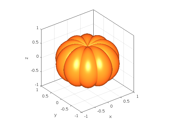

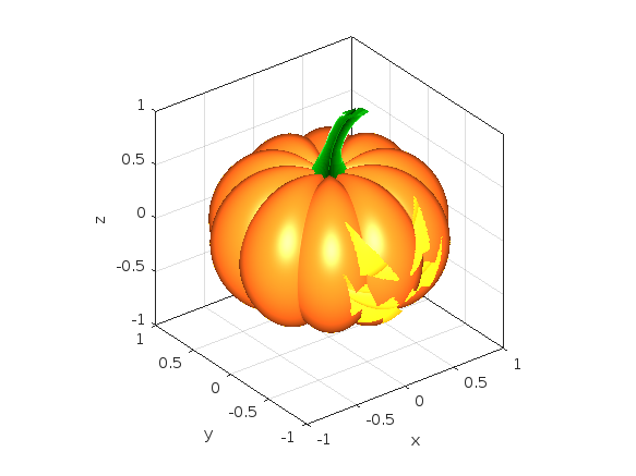
- The number of faces (n) controls the discretization of the pumpkin. The larger it is, the smoother the mask will be, but at the same time the computational cost will also increase. If you are using this for the contest which has a timeout limit of 235 seconds, you might need to adjust it accordingly.
- You will also need to restrict the Z-coordinates appropriately (Z>=0) so that the mask is only applied on the front side of the pumpkin.
- If you are animating the face mask (more information about this below), and you need the eyes and mouth to fully close at any point, avoid using the second argument of the inpolygon function that gives you the points located on the edge of the regions.

- Replace the legend with a colorbar to update the location and orientation of the colorbar.
- Define a GridSizeChangedFcn within the loop so that it is called every time a tile is added.
- Create a figure with many tiles (~20) and dynamically set a color to each row of axes.
- Assign xlabels only to the bottom row of tiles and ylabels to only the left column of tiles.
Starting in MATLAB R2022a, use the append option in exportgraphics to create GIF files from animated axes, figures, or other visualizations.
This basic template contains just two steps:
% 1. Create the initial image file
gifFile = 'myAnimation.gif';
exportgraphics(obj, gifFile);
% 2. Within a loop, append the gif image
for i = 1:20
      %   %   %   %   %   %    %
      % Update the figure/axes %
      %   %   %   %   %   %    %
exportgraphics(obj, gifFile, Append=true); end
Note, exportgraphics will not capture UI components such as buttons and knobs and requires constant axis limits.
To create animations of images or more elaborate graphics, learn how to use imwrite to create animated GIFs .
Share your MATLAB animated GIFs in the comments below!
See Also
This Community Highlight is attached as a live script
You've spent hours designing the perfect figure and now it's time to add it to a presentation or publication but the font sizes in the figure are too small to see for the people in the back of the room or too large for the figure space in the publication. You've got titles, subtitles, axis labels, legends, text objects, and other labels but their handles are inaccessible or scattered between several blocks of code. Making your figure readable no longer requires digging through your code and setting each text object's font size manually.
Starting in MATLAB R2022a, you have full control over a figure's font sizes and font units using the new fontsize function (see release notes ).
Use fontsize() to
- Set FontSize and FontUnits properties for all text within specified graphics objects
- Incrementally increase or decrease font sizes
- Specify a scaling factor to maintain relative font sizes
- Reset font sizes and font units to their default values . Note that the default font size and units may not be the same as the font sizes/units set directly with your code.
When specifying an object handle or an array of object handles, fontsize affects the font sizes and font units of text within all nested objects.
While you're at it, also check out the new fontname function that allows you to change the font name of objects in a figure!
Give the new fontsize function a test drive using the following demo figure in MATLAB R2022a or later and try the following commands:
% Increase all font sizes within the figure by a factor of 1.5
fontsize(fig, scale=1.5)
% Set all font sizes in the uipanel to 16
fontsize(uip, 16, "pixels")
% Incrementally increase the font sizes of the left two axes (x1.1)
% and incrementally decrease the font size of the legend (x0.9)
fontsize([ax1, ax2], "increase")
fontsize(leg, "decrease")
% Reset the font sizes within the entire figure to default values
fontsize(fig, "default")
% Create fake behavioral data
rng('default')
fy = @(a,x)a*exp(-(((x-8).^2)/(2*3.^2)));
x = 1 : 0.5 : 20;
y = fy(32,x);
ynoise = y+8*rand(size(y))-4;
selectedTrial = 13;
% Plot behavioral data
fig = figure('Units','normalized','Position',[0.1, 0.1, 0.4, 0.5]);
movegui(fig, 'center')
tcl = tiledlayout(fig,2,2);
ax1 = nexttile(tcl);
hold(ax1,'on')
h1 = plot(ax1, x, ynoise, 'bo', 'DisplayName', 'Response');
h2 = plot(ax1, x, y, 'r-', 'DisplayName', 'Expected');
grid(ax1, 'on')
title(ax1, 'Behavioral Results')
subtitle(ax1, sprintf('Trial %d', selectedTrial))
xlabel(ax1, 'Time (seconds)','Interpreter','Latex')
ylabel(ax1, 'Responds ($\frac{deg}{sec}$)','Interpreter','Latex')
leg = legend([h1,h2]);
% Plot behavioral error
ax2 = nexttile(tcl,3);
behavioralError = ynoise-y;
stem(ax2, x, behavioralError)
yline(ax2, mean(behavioralError), 'r--', 'Mean', ...
    'LabelVerticalAlignment','bottom')
grid(ax2, 'on')
title(ax2, 'Behavioral Error')
subtitle(ax2, ax1.Subtitle.String)
xlabel(ax2, ax1.XLabel.String,'Interpreter','Latex')
ylabel(ax2, 'Response - Expected ($\frac{deg}{sec}$)','Interpreter','Latex')
% Simulate spike train data
ntrials = 25;
nSamplesPerSecond = 3;
nSeconds = max(x) - min(x);
nSamples = ceil(nSeconds*nSamplesPerSecond);
xTime = linspace(min(x),max(x), nSamples);
spiketrain = round(fy(1, xTime)+(rand(ntrials,nSamples)-.5));
[trial, sample] = find(spiketrain);
time = xTime(sample);
% Spike raster plot
axTemp = nexttile(tcl, 2, [2,1]);
uip = uipanel(fig, 'Units', axTemp.Units, ...
    'Position', axTemp.Position, ...
    'Title', 'Neural activity', ...
    'BackgroundColor', 'W');
delete(axTemp)
tcl2 = tiledlayout(uip, 3, 1);
pax1 = nexttile(tcl2);
plot(pax1, time, trial, 'b.', 'MarkerSize', 4)
yline(pax1, selectedTrial-0.5, 'r-', ...
    ['\leftarrow Trial ',num2str(selectedTrial)], ...
    'LabelHorizontalAlignment','right', ...
    'FontSize', 8);
linkaxes([ax1, ax2, pax1], 'x')
pax1.YLimitMethod = 'tight';
title(pax1, 'Spike train')
xlabel(pax1, ax1.XLabel.String)
ylabel(pax1, 'Trial #')
% Show MRI
pax2 = nexttile(tcl2,2,[2,1]);
[I, cmap] = imread('mri.tif');
imshow(I,cmap,'Parent',pax2)
hold(pax2, 'on')
th = 0:0.1:2*pi;
plot(pax2, 7*sin(th)+84, 5*cos(th)+90, 'r-','LineWidth',2)
text(pax2, pax2.XLim(2), pax2.YLim(1), 'ML22a',...
    'FontWeight', 'bold', ...
    'Color','r', ...
    'VerticalAlignment', 'top', ...
    'HorizontalAlignment', 'right', ...
    'BackgroundColor',[1 0.95 0.95])
title(pax2, 'Area of activation')
% Overall figure title
title(tcl, 'Single trial responses')
This Community Highlight is attached as a live script.