predict
Classify observations using naive Bayes classifier
Description
[
also returns the Posterior Probability (label,Posterior,Cost]
= predict(Mdl,X)Posterior) and predicted
(expected) Misclassification Cost (Cost) corresponding to
the observations (rows) in Mdl.X. For each observation in
X, the predicted class label corresponds to the minimum
expected classification cost among all classes.
Examples
Label Test Sample Observations of Naive Bayes Classifier
Load the fisheriris data set. Create X as a numeric matrix that contains four petal measurements for 150 irises. Create Y as a cell array of character vectors that contains the corresponding iris species.
load fisheriris
X = meas;
Y = species;
rng('default')  % for reproducibility
Randomly partition observations into a training set and a test set with stratification, using the class information in Y. Specify a 30% holdout sample for testing.
cv = cvpartition(Y,'HoldOut',0.30);Extract the training and test indices.
trainInds = training(cv);
testInds = test(cv);
Specify the training and test data sets.
XTrain = X(trainInds,:);
YTrain = Y(trainInds);
XTest = X(testInds,:);
YTest = Y(testInds);
Train a naive Bayes classifier using the predictors XTrain and class labels YTrain. A recommended practice is to specify the class names. fitcnb assumes that each predictor is conditionally and normally distributed.
Mdl = fitcnb(XTrain,YTrain,'ClassNames',{'setosa','versicolor','virginica'})
Mdl =
  ClassificationNaiveBayes
              ResponseName: 'Y'
     CategoricalPredictors: []
                ClassNames: {'setosa'  'versicolor'  'virginica'}
            ScoreTransform: 'none'
           NumObservations: 105
         DistributionNames: {'normal'  'normal'  'normal'  'normal'}
    DistributionParameters: {3x4 cell}
Mdl is a trained ClassificationNaiveBayes classifier.
Predict the test sample labels.
idx = randsample(sum(testInds),10);
label = predict(Mdl,XTest);
Display the results for a random set of 10 observations in the test sample.
table(YTest(idx),label(idx),'VariableNames',...
    {'TrueLabel','PredictedLabel'})
ans=10×2 table
      TrueLabel       PredictedLabel
    ______________    ______________

    {'virginica' }    {'virginica' }
    {'versicolor'}    {'versicolor'}
    {'versicolor'}    {'versicolor'}
    {'virginica' }    {'virginica' }
    {'setosa'    }    {'setosa'    }
    {'virginica' }    {'virginica' }
    {'setosa'    }    {'setosa'    }
    {'versicolor'}    {'versicolor'}
    {'versicolor'}    {'virginica' }
    {'versicolor'}    {'versicolor'}
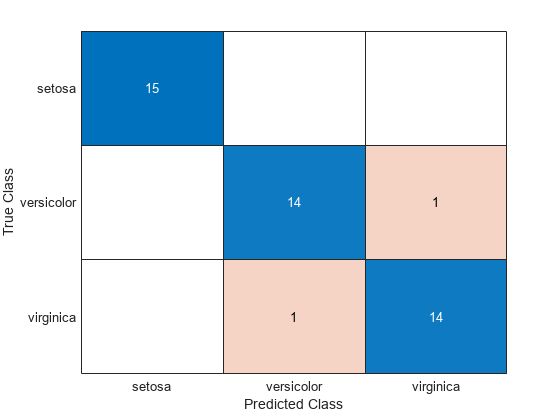
Create a confusion chart from the true labels YTest and the predicted labels label.
cm = confusionchart(YTest,label);
Estimate Posterior Probabilities and Misclassification Costs
Estimate posterior probabilities and misclassification costs for new observations using a naive Bayes classifier. Classify new observations using a memory-efficient pretrained classifier.
Load the fisheriris data set. Create X as a numeric matrix that contains four petal measurements for 150 irises. Create Y as a cell array of character vectors that contains the corresponding iris species.
load fisheriris
X = meas;
Y = species;
rng('default')  % for reproducibility
Partition the data set into two sets: one contains the training set, and the other contains new, unobserved data. Reserve 10 observations for the new data set.
n = size(X,1);
newInds = randsample(n,10);
inds = ~ismember(1:n,newInds);
XNew = X(newInds,:);
YNew = Y(newInds);
Train a naive Bayes classifier using the predictors X and class labels Y. A recommended practice is to specify the class names. fitcnb assumes that each predictor is conditionally and normally distributed.
Mdl = fitcnb(X(inds,:),Y(inds),...
    'ClassNames',{'setosa','versicolor','virginica'});
Mdl is a trained ClassificationNaiveBayes classifier.
Conserve memory by reducing the size of the trained naive Bayes classifier.
CMdl = compact(Mdl);
whos('Mdl','CMdl')
  Name      Size            Bytes  Class                                                        Attributes

  CMdl      1x1              5575  classreg.learning.classif.CompactClassificationNaiveBayes
  Mdl       1x1             12900  ClassificationNaiveBayes
CMdl is a CompactClassificationNaiveBayes classifier. It uses less memory than Mdl because Mdl stores the data.
Display the class names of CMdl using dot notation.
CMdl.ClassNames
ans = 3x1 cell
    {'setosa'    }
    {'versicolor'}
    {'virginica' }
Predict the labels. Estimate the posterior probabilities and expected class misclassification costs.
[labels,PostProbs,MisClassCost] = predict(CMdl,XNew);
Compare the true labels with the predicted labels.
table(YNew,labels,PostProbs,MisClassCost,'VariableNames',...
    {'TrueLabels','PredictedLabels',...
    'PosteriorProbabilities','MisclassificationCosts'})
ans=10×4 table
      TrueLabels      PredictedLabels             PosteriorProbabilities                      MisclassificationCosts
    ______________    _______________    _________________________________________    ______________________________________

    {'virginica' }    {'virginica' }     4.0832e-268     4.6422e-09              1             1             1    4.6422e-09
    {'setosa'    }    {'setosa'    }               1     3.0706e-18     4.6719e-25    3.0706e-18             1             1
    {'virginica' }    {'virginica' }     1.0007e-246     5.8758e-10              1             1             1    5.8758e-10
    {'versicolor'}    {'versicolor'}      1.2022e-61        0.99995     4.9859e-05             1    4.9859e-05       0.99995
    {'virginica' }    {'virginica' }      2.687e-226     1.7905e-08              1             1             1    1.7905e-08
    {'versicolor'}    {'versicolor'}      3.3431e-76        0.99971     0.00028983             1    0.00028983       0.99971
    {'virginica' }    {'virginica' }       4.05e-166      0.0028527        0.99715             1       0.99715     0.0028527
    {'setosa'    }    {'setosa'    }               1     1.1272e-14     2.0308e-23    1.1272e-14             1             1
    {'virginica' }    {'virginica' }     1.3292e-228     8.3604e-10              1             1             1    8.3604e-10
    {'setosa'    }    {'setosa'    }               1     4.5023e-17     2.1724e-24    4.5023e-17             1             1
PostProbs and MisClassCost are 10-by-3 numeric matrices, where each row corresponds to a new observation and each column corresponds to a class. The order of the columns corresponds to the order of CMdl.ClassNames.
Plot Posterior Probability Regions for Naive Bayes Classifier
Load the fisheriris data set. Create X as a numeric matrix that contains petal length and width measurements for 150 irises. Create Y as a cell array of character vectors that contains the corresponding iris species.
load fisheriris
X = meas(:,3:4);
Y = species;
Train a naive Bayes classifier using the predictors X and class labels Y. A recommended practice is to specify the class names. fitcnb assumes that each predictor is conditionally and normally distributed.
Mdl = fitcnb(X,Y,'ClassNames',{'setosa','versicolor','virginica'});
Mdl is a trained ClassificationNaiveBayes classifier.
Define a grid of values in the observed predictor space.
xMax = max(X);
xMin = min(X);
h = 0.01;
[x1Grid,x2Grid] = meshgrid(xMin(1):h:xMax(1),xMin(2):h:xMax(2));
Predict the posterior probabilities for each instance in the grid.
[~,PosteriorRegion] = predict(Mdl,[x1Grid(:),x2Grid(:)]);
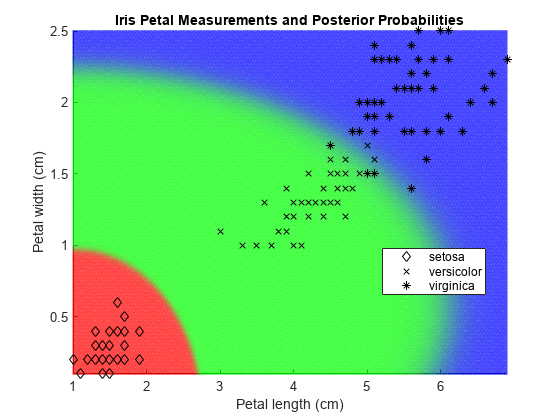
Plot the posterior probability regions and the training data.
h = scatter(x1Grid(:),x2Grid(:),1,PosteriorRegion);
h.MarkerEdgeAlpha = 0.3;
Plot the data.
hold on
gh = gscatter(X(:,1),X(:,2),Y,'k','dx*');
title 'Iris Petal Measurements and Posterior Probabilities';
xlabel 'Petal length (cm)';
ylabel 'Petal width (cm)';
axis tight
legend(gh,'Location','Best')
hold off
Input Arguments
Output Arguments
More About
Alternative Functionality
Simulink Block
To integrate the prediction of a naive Bayes classification model into Simulink®, you can use the ClassificationNaiveBayes Predict block in the Statistics and Machine Learning Toolbox™ library or a MATLAB® Function block with the predict function. For
examples, see Predict Class Labels Using ClassificationNaiveBayes Predict Block and Predict Class Labels Using MATLAB Function Block.
When deciding which approach to use, consider the following:
If you use the Statistics and Machine Learning Toolbox library block, you can use the Fixed-Point Tool (Fixed-Point Designer) to convert a floating-point model to fixed point.
Support for variable-size arrays must be enabled for a MATLAB Function block with the
predictfunction.If you use a MATLAB Function block, you can use MATLAB functions for preprocessing or post-processing before or after predictions in the same MATLAB Function block.
Extended Capabilities
Version History
Introduced in R2014b
You can also select a web site from the following list:
Americas
- América Latina (Español)
- Canada (English)
- United States (English)
Europe
- Belgium (English)
- Denmark (English)
- Deutschland (Deutsch)
- España (Español)
- Finland (English)
- France (Français)
- Ireland (English)
- Italia (Italiano)
- Luxembourg (English)
- Netherlands (English)
- Norway (English)
- Österreich (Deutsch)
- Portugal (English)
- Sweden (English)
- Switzerland
- United Kingdom (English)