Solver Profiler

R2026b

Identify solver performance bottlenecks

Description

The Solver Profiler logs and analyzes solver activity, such as zero-crossing events and solver resets, in a simulation. These solver events are necessary for accurate simulation but incur computational cost. Profiling the solver activity helps identify configuration and modeling issues that cause solver events to occur more frequently than necessary.

The Solver Profiler provides recommendations for configuration and modeling changes that can speed up simulations by reducing the number of solver events. The profiling results include statistical and graphical information about these solver events:

• Zero-crossing events

• Solver exceptions

• Solver resets

• Jacobian computations

To simplify and speed up performance analysis, generate AI explanations of profiling results. The AI explanation summarizes key findings, identifies potential bottlenecks, and provides actionable recommendations to improve simulation performance. To analyze profiling results using AI, you must have a Simulink^® Copilot license. (since R2026b)

Local Solver Profiler

Since R2026b

The Local Solver Profiler configures profiling settings and displays profiling results for a local solver. The Local Solver Profiler provides the same configuration and visualization options as the Solver Profiler. However, the Local Solver Profiler toolstrip does not include the simulation controls that the Solver Profiler provides in the Profile section. To profile one or more local solvers, use the Local Solver Analyzer.

For more information, see Local Solver Analyzer.

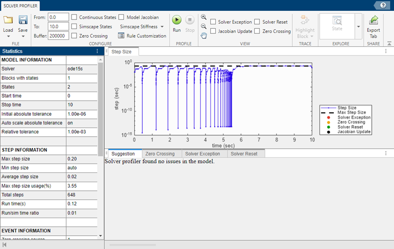
Open the Solver Profiler

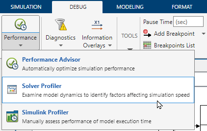
• Simulink Toolstrip: On the Debug tab, click the Performance button arrow and select Solver Profiler.

  

• Solver information menu: To open the Solver information menu, click the hyperlink on the right of the status bar at the bottom of the Simulink Editor. Then, click Solver Profiler .

  

• MATLAB^® Command Window: solverprofiler.profileModel(mdl,OpenSP="on") profiles the solver for the model mdl and opens the Solver Profiler after the simulation completes.

Examples

Identify Source of Zero Crossing Event

Open the example, which contains a model named BouncingBallWithSwitch.

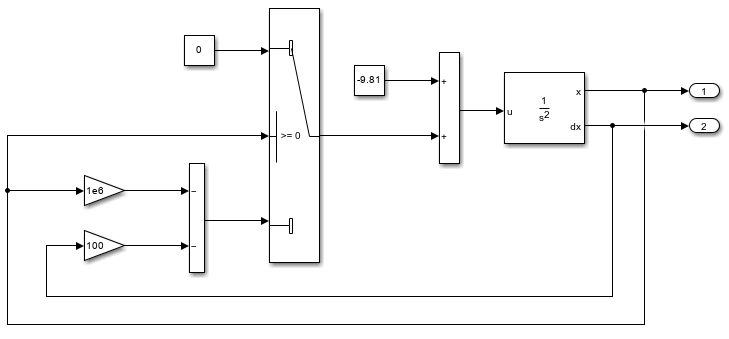
Open the Solver Profiler. In the Simulink® Toolstrip, on the Debug tab, in the Performance section, click the Performance button arrow and select Solver Profiler.

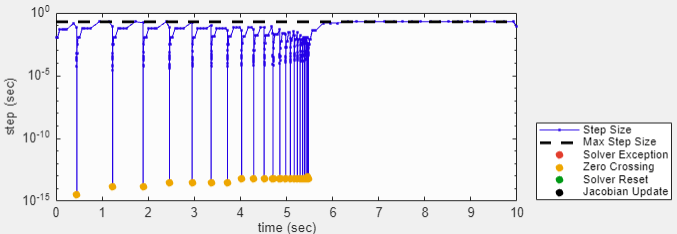
To run a profiling simulation, in the Solver Profiler, click Run. The Solver Profiler collects information about solver events that occur during the profiling simulation. When the simulation completes, the Solver Profiler displays information in the Statistics pane and a plot of the step size calculated for each step of the simulation.

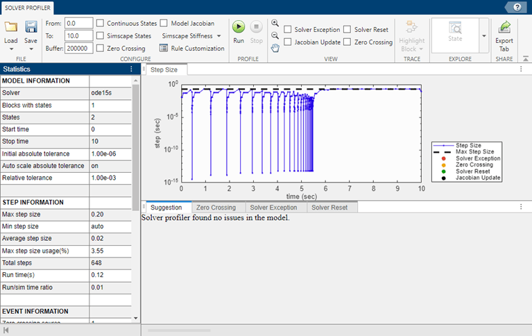
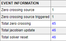
In the Statistics pane, scroll down to view the event information, which shows that 45 zero-crossing events occurred during simulation from one source.

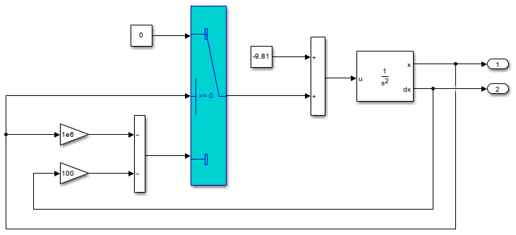
To view information about the source of the zero-crossing events, select the Zero Crossing tab. The zero crossing events come from the Switch block.

To annotate the plot of the step sizes with the zero-crossing events, in the Statistics pane, click the value for the Total Zero Crossings row. The yellow dots indicate when each zero crossing occurred. Where the zero crossings occurred, the step size decreased significantly.

To highlight in the block diagram the Switch block that produced the zero crossings, on the Zero Crossing tab, select the block path. Then, in the Trace section, click Highlight Block.

Analyze Profiling Results Using AI

Since R2026b

Simplify and speed up performance analysis by using AI to explain profiling results. To generate the AI explanation:

1. Open the Solver Profiler. In the Simulink Toolstrip, on the Debug tab, click the Performance button arrow and select Solver Profiler.

2. Profile a simulation. In the toolstrip, under Profile, click Run.

3. After the profiling simulation completes, generate the AI explanation. In the toolstrip, in the Explain section, click Explain with AI.

The Solver Profiler displays the AI explanation in the bottom panel on the Explain with AI tab. The explanation provides an overview of the profiling results, highlights specific insights, and summarizes key details from the results.

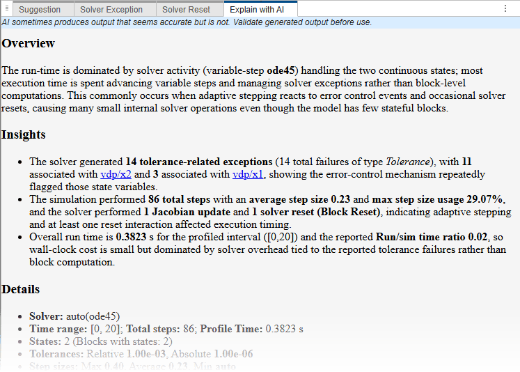
The AI explanation provides insight into the solver activity during simulation even when the Solver Profiler does not identify any issues in the model design or configuration.

Configure Profiling Settings for Local Solvers

By default, the options you specify in the Configure section of the Solver Profiler toolstrip apply to the top solver and the selected local solvers. To specify different profiling options for a local solver, use the Local Solver Profiler.

1. Open the Local Solver Analyzer. In the Solver Profiler toolstrip, in the Analyze section, click Local Solver.

2. In the Model Hierarchy pane, select the node of the referenced model that uses the local solver.

3. Open an instance of the Local Solver Profiler for the selected referenced model. In the right pane, click Open Local Solver Profiler to configure settings for new profiling simulation .

4. In the Local Solver Profiler, specify the profiling options for the local solver.

The options you specify in the Local Solver Profiler apply to only the selected referenced model. To specify different profiling options for more than one local solver, open an instance of the Local Solver Profiler for each referenced model.

To profile local solvers using the specified settings, in the Local Solver Analyzer, click Run.

Related Examples

• Examine Model Dynamics Using Solver Profiler
• Solver Resets
• Zero-Crossing Events
• Solver Exception Events
• Analyze Jacobian Updates Using Solver Profiler

Parameters

Configure

From — Profiling start time

model start time (default) | scalar

The time at which the Solver Profiler starts logging solver data during simulation, specified in seconds. By default, the Solver Profiler logs data from the start of the simulation.

This parameter does not specify the start time of the simulation or modify the Start time configuration parameter in the model.

To — Profiling stop time

model stop time (default) | scalar

The time at which the Solver Profiler stops profiling, specified in seconds. By default, the profiling stop time is the same as the simulation stop time specified in the model. The simulation ends when it reaches the profiling stop time or the simulation stop time, whichever occurs first.

This parameter does not modify the Stop time configuration parameter in the model.

Buffer — Maximum number of logged solver events

50000 (default) | positive scalar

Maximum number of events that are logged. If the number of logged events reaches this value and memory is available, increase BufferSize. If memory is limited, consider lowering the value.

Continuous States — Option to save continuous states for analysis

off (default) | on

To save continuous states for analysis in the Solver Profiler and State Explorer, select this parameter. By default, the Solver Profiler does not save continuous states.

Note

To reduce overhead, the Solver Profiler compresses states data. The logged results support solver analysis but the state values might not be exact. To log and analyze precise state values, enable states logging. In the Configuration Parameters dialog box, on the Data Import/Export pane, select States.

Simscape States — Option to save Simscape™ states for analysis

off (default) | on

To save Simscape states for analysis in the Solver Profiler and Simscape Results Explorer (Simscape), select this parameter. By default, the Solver Profiler does not save Simscape states.

Zero Crossing — Option to save zero-crossing data for analysis

off (default) | on

To save zero-crossing data for analysis in the Solver Profiler and Zero Crossing Explorer, select this parameter. By default, the Solver Profiler does not save zero-crossing data.

Model Jacobian — Option to save model Jacobian for analysis

off (default) | on

To save solver Jacobian matrices for analysis in the Solver Profiler, select this parameter. This option is useful for simulations that use implicit solvers. For a comparison of solvers, see Compare Solvers.

For a more detailed explanation of the solver Jacobian, see Choose Jacobian Method for Implicit Solvers.

Simscape Stiffness — Option to save stiffness analysis of Simscape states

array

To save stiffness analysis of Simscape states for analysis in the Solver Profiler, select this parameter and specify an array of time points at which to capture the data.

For more information, see How Simscape Models Represent Physical Systems (Simscape).

Rule Customization — Profiler rules and threshold settings

off (default) | on

To access the rule set, click Rule Customization in the Solver Profiler. You can select which rules you want to apply and specify the thresholds for most of the built-in rules. To modify the threshold for a rule, enable the rule. Then, enter the desired threshold value.

Custom Rule Set

To override or extend the built-in rule, specify a custom rule set.

1. Define the custom rule set in a MATLAB function.

2. In the Rule Set dialog box, in the Custom Rule section, select the check box. Then, enter the name of the function that defines the custom rule set.

For example, this code defines a custom rule set using a function named customRule. The input to the function is a structure that contains the profiling data. The function implements a rule that checks whether any zero-crossing events occurred during the profiling simulation.

function diagnosticsString = customRule(profilerData)
    if isempty(profilerData.zcEvents)
        diagnosticsString{1} = "No zero crossing event detected.";
    else
        diagnosticsString{1} = "Zero-crossing events detected.";
    end
end

The table summarizes the fields in the structure of profiling data you can use to implement custom rules.

Field	Value
stateInfo — Block state information	Structure that contains these fields: name — Block name value — State values blockIdx — Block ID
blockInfo — Blocks and state IDs	Structure that contains these fields: name — Block name stateIdx — State ID
zcSrcInfo — Blocks that cause zero crossings	Structure that contains these fields: name — Block name blockIdx — Block ID
zcEvents — Zero-crossing event times and state IDs	Structure that contains these fields: t — Event time srcIdx — Block ID
exceptionEvents — Solver exception event times, state IDs, and causes	Structure that contains these fields: t — Event time stateIdx — State ID cause — Cause of exception
resetTime — Solver reset times	Array of solver reset times
tout — Simulation times	Array of simulation time steps

View

Solver Exception — Option to show solver exception events

off (default) | on

To highlight solver exception events in the step size plot, select this parameter.

Solver Reset — Option to show solver reset events

off (default) | on

To highlight solver reset events in the step size plot, select this parameter.

Jacobian Update — Option to show Jacobian update events

off (default) | on

To highlight Jacobian update events in the step size plot, select this parameter.

Zero Crossing — Option to show zero-crossing events

off (default) | on

To highlight zero-crossing events in the step size plot, select this parameter.

Tips

• When you want to analyze and improve simulation performance, consider starting the analysis by analyzing your model and simulation configuration using the Performance Advisor.

• After analyzing the model and simulation configuration using the Performance Advisor, you can perform deeper analysis by profiling simulations using the Solver Profiler and the Simulink Profiler.

  • The Solver Profiler analyzes the performance of the selected solver for the model, which can be particularly helpful for simulations that use variable-step solvers. The profiling results help you identify when and why the step size is limited.

  • The Simulink Profiler helps you identify bottlenecks for simulation performance by analyzing the distribution of simulation execution time among model components.

Version History

Introduced in R2016a

R2026b: Local Solver Analyzer: Configure and profile local solvers in model hierarchies

Using the Local Solver Analyzer, you can:

• Visualize a model reference hierarchy.

• Enable, disable, and configure local solvers in referenced models.

• Profile one or more local solvers in the model hierarchy.

To open the Local Solver Analyzer, open the Solver Profiler. Then, in the toolstrip, in the Analyze section, click Local Solver.

When you profile local solvers, the Local Solver Analyzer displays a summary of the profiling results. To analyze the profiling results, view the profiling data in the Local Solver Profiler. The Local Solver Profiler provides the same data and visualizations as the Solver Profiler but does not support running profiling simulations. To profile a local solver, you must simulate the top model.

R2026b: Analyze profiling results using AI

If you have a Simulink Copilot license, you can generate AI explanations of Solver Profiler results. The AI explanation summarizes key findings, identifies potential bottlenecks, and provides actionable recommendations to improve simulation performance.