Spectrum Analyzer

R2026b

Display frequency spectrum of time-domain signals

• 

Spectrum Analyzer block

To add a block to a model, double-click the canvas and start typing the block name. Then, select the block from the list.

Libraries:
RF Blockset / Circuit Envelope / Utilities

Description

Note

The Spectrum Analyzer block in RF Blockset™ provides a subset of the functionality provided by the DSP System Toolbox™ block with the same name. This page describes the block configuration and functionality available with a RF Blockset license.

If you also have a DSP System Toolbox license, then the Spectrum Analyzer block in the RF Blockset > Utilities library is identical to the block in the DSP System Toolbox > Sinks library. For more information, see Spectrum Analyzer (DSP System Toolbox).

The Spectrum Analyzer block displays frequency spectra of input signals with discrete sample times.

In a RF Blockset model, to use a Spectrum Analyzer block instead of a regular scope:

1. Add a Spectrum Analyzer block to your block diagram.

2. If your model uses a variable-step solver, also add a Rate Transition block and connect it to the input port of the Spectrum Analyzer block. Set the Output port sample time parameter to the sample time you want the Spectrum Analyzer to use.

   If your model uses a local solver, then it outputs physical signals with discrete sample times and you do not need to add a Rate Transition block. However, if you need to downsample from the solver fixed step size, you can use a Rate Transition block. For more information on using local solvers, see Making Optimal Solver Choices for Physical Simulation.

3. Use a PS-Simulink Converter block to connect the physical output signal of interest to the input port of the Spectrum Analyzer block (or to the input port of the Rate Transition block, if you are using one). For more information, see Connecting Simscape Diagrams to Simulink Sources and Scopes. You can also use additional signal processing blocks between the PS-Simulink Converter and the Spectrum Analyzer blocks to enhance signal quality.

4. Run the simulation. Once the simulation is complete, the Spectrum Analyzer, referred to here as the scope, opens and displays the frequency spectrum of the signal.

Programmatic Control

You can configure and display the Spectrum Analyzer settings from the command line with the SpectrumAnalyzerBlockConfiguration object.

Examples

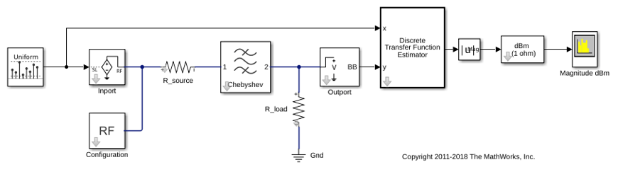
Analysis of Frequency Response of RF System

Analyze the frequency response of an RF system.

• Open Script

Ports

Input

u — Signals to visualize

scalar | vector | matrix | array

Connect the signals you want to visualize. You can have up to 96 input ports. Input signals must have these characteristics:

• Signal Domain — Frequency or time signals.

• Type — Discrete signals.

• Data type — Any data type that Simulink^® supports. See Data Types Supported by Simulink.

• Dimension — One dimensional (vector), two dimensional (matrix), or multidimensional (array) signals. Input signal must have a fixed number of channels. See Signal Dimensions and Determine Signal Dimensions.

The Spectrum Analyzer block supports variable-size input signals, that is, the frame size of the signals can change during simulation. When the signal frame size changes, the sample rate the scope uses changes accordingly, which in turn updates the frequency span of the spectrum display.

The Spectrum Analyzer block accepts fixed-point input, but converts it to double for display.

This port is unnamed until you enable the RBW port. (since R2024a)

Data Types: single | double | int8 | int16 | int32 | int64 | uint8 | uint16 | uint32 | uint64 | fixed point
Complex Number Support: Yes

RBW — RBW Value

positive scalar

Specify the resolution bandwidth in Hz through this port. RBW defines the smallest positive frequency that can be resolved by the scope. You can also specify the RBW value using the RBW (Hz) parameter on the Estimation tab.

Dependencies

To enable this port, set RBW (Hz) to Input port on the Estimation tab.

Data Types: single | double | int8 | int16 | int32 | int64 | uint8 | uint16 | uint32 | uint64 | Boolean | fixed point

Parameters

This section lists the block parameters for the Spectrum Analyzer block in Simscape™ and RF Blockset. For a complete list of parameters, see Spectrum Analyzer (DSP System Toolbox).

Home Tab

Views

Display Settings — Set configuration and style settings

button

Click the Display Settings button to customize the Display Settings.

Display Settings

Num Inputs — Number of input ports

1 (default) | integer between 1 and 96

The number of input ports to the block, specified as an integer between 1 and 96. To change the number of input ports, drag a new input signal line to the block and the block automatically creates new ports.

Programmatic Use

Block Parameter: NumInputPorts

Type: character vector or string scalar

Values: scalar between 1 and 96

Open at Simulation Start — Automatically open scope when simulation starts

on (default) | off

Select this parameter to automatically open the Spectrum Analyzer window when you run the simulation.

Tunable: Yes

Programmatic Use

Block Parameter: OpenAtSimulationStart

Type: logical

Display Precision — Precision of data in scope display

4 (default) | positive integer ≤ 15

Since R2024b

Specify the precision of numeric values in the scope display as a positive integer in the range [1, 15].

Tunable: Yes

Y-Label — y-axis label

character vector | string scalar

Specify the y-axis label in the Spectrum display as a character vector or a string scalar. To display signal units, add (%<SignalUnits>) to the label. When simulation starts, Simulink replaces (%SignalUnits) with the units associated with the signals.

For example, for a velocity signal with units of m/s enter

Velocity (%<SignalUnits>)

Tunable: Yes

Programmatic Use

Block Parameter: YLabel

Type: character vector or string scalar

Automatically Scale Axes Limits — Option to automatically scale y-axis limits

on (default) | off

Since R2026a

Select this parameter to automatically scale the y-axis limits of the spectrum analyzer display. When you clear this parameter, you can manually specify the axes limits using the Y-Limits parameter.

To enable the Color Limits parameter, you must have a DSP System Toolbox license.

Programmatic Use

Block Parameter: AxesScaling

Type: logical

Y-Limits — y-axis limits

[−80 20] | [ymin ymax]

Specify the y-axis limits in the Spectrum Analyzer display as a two-element numeric vector of the form [ymin ymax]. The units of the y-axis limits depend on the Spectrum Unit in the Home tab.

Tunable: Yes

Dependencies

To enable this parameter, clear the Automatically Scale Axes Limits parameter in the Display Settings > Display and Labels. (since R2026a)

Programmatic Use

Block Parameter: YLimits

Type: double

Title — Display title

character vector | string

Specify the display title. Enter %<SignalLabel> to use the signal labels in the Simulink model as the axes titles.

Tunable: Yes

Programmatic Use

Block Parameter: Title

Type: character vector or string

Show Grid — Show internal grid lines

on (default) | off

Select this check box to show the grid in the Spectrum Analyzer display.

Tunable: Yes

Programmatic Use

Block Parameter: ShowGrid

Type: logical

Font Size — Font size of labels

8.5 (default) | positive scalar

Specify the font size of the ticks, labels, title, and measurements of the scope as a positive scalar.

Tunable: Yes

Background Color — Window background

black (default) | color picker

Specify the background color in the scope figure.

Tunable: Yes

Axes Color — Axes background color

black (default) | color picker

Specify the background color of the axes.

Tunable: Yes

Labels Color — Color of labels

gray (default) | color picker

Specify the color of the labels, grid, and the channel names in the legend.

Tunable: Yes

Line Selector — Channel for line property settings

channel names

Specify the channel for which you want to modify the visibility, line color, style, width, and marker properties.

Tunable: Yes

Line Visible — Channel visibility

on (default) | off

Select this check box to display the channel you have selected. If you clear this check box, the selected channel is no longer visible. You can also click the signal name in the legend to control its visibility.

Tunable: Yes

Line Style — Line style

- (default) | : | -. | -- | None

Specify the line style for the selected channel.

Tunable: Yes

Line Width — Line width

1.5 (default) | 0.5 | 1 | 2 | ...

Specify the line width for the selected channel.

Tunable: Yes

Plot Type — Plot type

Line (default) | Stem

Specify whether to display a Line or Stem plot in the Spectrum display.

You can individually control the type of plot for each channel. To control the type of plot for each channel, select the channel and set the Plot Type parameter accordingly. (since R2025a)

Tunable: Yes

Programmatic Use

Block Parameter: PlotType

Type: character vector or string scalar

Line Marker — Data point markers

None (default) | + | x | ...

Specify a data point marker for the selected channel. This parameter is similar to the Marker property for plots. You can choose any of the marker symbols from the drop-down list.

Tunable: Yes

Line Color — Line color

yellow (default) | color picker

Specify the line color for the selected channel.

Tunable: Yes

Frequency Settings

Sample Rate (Hz) — Sample rate the scope uses in Hz

Inherited (default) | positive scalar

Specify the sample rate the scope uses in Hz as one of the following:

• Inherited — Use this option to specify the same sample rate as the input signal.

• Positive scalar — The sample rate you specify must be at least the sample rate of the input signal.

When the signal frame size changes, the sample rate the scope uses changes accordingly, which in turn updates the frequency span of the spectrum display.

To display the sample rate on the status bar, click the $$⋮$$ icon in the status bar and select Sample Rate (Fs).

Programmatic Use

Block Parameter: SampleRate, SampleRateSource

Type: double

Tunable: Yes

Frequency Scale — Scale of frequency axis

Linear (default) | Log

Specify the scale to display frequencies as Linear or Log. When the frequency span contains negative frequency values, you cannot choose the logarithmic option.

Tunable: Yes

Programmatic Use

Block Parameter: FrequencyScale

Type: character vector or string scalar

Frequency Span — Frequency span settings

drop-down

Click the Frequency Span drop-down arrow to customize the frequency span settings.

Frequency Span Settings

Two-Sided Spectrum — Show two-sided spectrum

off (default) | on

Select this check box to show the two-sided spectrum. In this view, the spectrum analyzer shows both negative and positive frequencies. When the input signal is complex-valued, you must select this parameter. If you clear this check box, the spectrum analyzer shows a one-sided spectrum with positive frequencies only. In this case, the input signal data must be real valued.

When you clear this check box, the spectrum analyzer uses power folding. The y-axis values are twice the amplitude that they would be if you were to select this parameter, except at 0 and the Nyquist frequency. A one-sided power spectral density (PSD) contains the total power of the signal in the frequency interval from DC to half the Nyquist rate. For more information, see pwelch (Signal Processing Toolbox).

Tunable: Yes

Programmatic Use

Block Parameter: PlotAsTwoSidedSpectrum

Type: logical

Frequency Offset (Hz) — Offset to apply to frequency axis

0 (default) | scalar | vector

Specify the offset to apply to the frequency axis (x-axis) in units of Hz as one of the following:

• Scalar — Apply the same frequency offset to all channels.

• Vector — Apply a specific frequency offset for each channel. The vector length must be equal to the number of input channels.

  The overall span must fall within the Nyquist Frequency Interval.

Tunable: Yes

Programmatic Use

Block Parameter: FrequencyOffset

Type: double

Scale

Spectrum Type — Type of spectrum display

Power (default) | Power Density | RMS

Set the type of spectrum to display as one of these values:

• Power — Spectrum analyzer shows the power spectrum.

• Power Density — Spectrum analyzer shows the power spectral density. The power spectral density is the squared magnitude of the spectrum normalized to a bandwidth of 1 Hz.

• RMS — Spectrum analyzer shows the root mean square of the spectrum. The root-mean-square shows the square root of the mean square. Use this option to view the frequency of voltage or current signals.

Tunable: Yes

Programmatic Use

Block Parameter: SpectrumType

Type: character vector or string scalar

Data Types: char | string

Spectrum Unit — Units of the spectrum

dBm (default) | dBm/Hz | dBV | dBuV (since R2023b) | Vrms

Specify the units in which the spectrum analyzer displays the power values as one of the following:

• dBm

• dBV

• dBuV (since R2023b)

• Vrms

• dBm/Hz

Tunable: Yes

Dependencies

The units available depend on the value you choose for the Spectrum Type parameter in the Home tab.

Home tab > Spectrum Type option	Available Units
Power	dBm
Power Density	dBm/Hz
RMS	dBV, dBuV (since R2023b), Vrms

Programmatic Use

Block Parameter: SpectrumUnits

Type: character vector or string scalar

Scale — Scale options

drop-down

Click the Scale drop-down arrow to customize the scale options.

Scale Options

Reference load (Ω) — Reference load in Ω

1 (default) | positive real scalar

Specify the reference load in ohms that the spectrum analyzer uses as a reference to compute the power values.

Tunable: Yes

Dependencies

To enable this parameter, set the Spectrum Type to Power or Power Density in the Home tab.

Programmatic Use

Block Parameter: ReferenceLoad

Type: double

Export

Print — Print display

button

Click this button to save the scope display as an image or a PDF or to print the display.

Print to Figure — Print to MATLAB^® figure

button

Since R2026b

Click this button to print the scope window to MATLAB figure.

Copy to Clipboard — Send display to clipboard

button

Click this button to copy the scope display to the clipboard. You can preserve the color in the display by selecting Preserve Colors in the Copy to Clipboard drop down.

Preserve Colors — Preserve colors when copying to clipboard

off (default) | on

When you copy the display to the clipboard using the Copy to Clipboard and the Print options in the Home tab > Export section, select this parameter for the scope to preserve the colors.

To access Preserve Colors, click the drop-down arrow for Copy to Clipboard.

Tunable: Yes

Estimation Tab

Frequency Resolution

RBW (Hz) — Resolution bandwidth in Hz

Auto (default) | Input port | positive scalar

Specify the resolution bandwidth in Hz. This parameter defines the smallest positive frequency that can be resolved by the scope. By default, this parameter is set to Auto. In this case, the spectrum analyzer determines the appropriate value to ensure that there are 1024 RBW intervals over the specified frequency span.

If you set this parameter to Input port, you can specify the RBW value through the RBW input port on the block.

If you set this parameter to a numeric value, the value must allow at least two RBW intervals over the specified frequency span. In other words, the ratio of the overall frequency span to RBW must be greater than two:

$$\frac{span}{RBW}>2$$

To display this property on the status bar, click the $$⋮$$ icon in the status bar and select RBW.

Programmatic Use

Block Parameter: RBWSource, RBW

Type: character vector, string scalar, double

Tunable: Yes

Window — Window options

drop-down

Click the Window drop-down arrow to customize the window options.

Window Options

Window — Windowing method

Hann (default) | Rectangular

Specify the windowing method to apply to the spectrum. Windowing is used to control the effect of sidelobes in spectral estimation. The window you specify affects the window length required to achieve a resolution bandwidth and the required number of samples per update. For more information about windowing, see Windows (Signal Processing Toolbox).

You can access additional windowing algorithms using DSP System Toolbox.

Tunable: Yes

Programmatic Use

Block Parameter: Window

Type: character vector or string scalar

Window Invariant Samples Per Update — Maintain samples per update

off (default) | on

Select this parameter to maintain the number of samples per update N_samples at 1024 regardless of the window you select. The RBW value adjusts according to the window you select.

$$N_{samples}=\frac{\left(1-\frac{O_p}{100}\right)\times NENBW\times F_s}{RBW},$$

where:

• O_p is the overlap percentage you specify in the Overlap (%) parameter.

• Fs is the sample rate you specify in the Sample Rate (Hz) parameter.

• RBW is the resolution bandwidth you specify in the RBW (Hz) parameter.

• NENBW is the normalized effective noise bandwidth. For more information, see Normalized Effective Noise Bandwidth (NENBW).

When you clear this parameter, the scope maintains the same RBW value and adjusts the number of samples required per update N_samples depending on the window you select.

Programmatic Use

Block Parameter: WindowInvariantSamplesPerUpdate

Type: logical

Tunable: Yes

Overlap (%) — Percentage of overlap

0 (default) | scalar in the range [0 100)

Specify the percentage of overlap between the previous and the current buffered data segments as a scalar in the range [0 100). The overlap creates a window segment that the scope uses to compute a spectral estimate. The value must be greater than or equal to zero and less than 100.

Tunable: Yes

Programmatic Use

Block Parameter: OverlapPercent

Type: double

Averaging

Averaging Method — Smoothing method

Exponential (default) | VBW | Running

Specify the smoothing method as one of the following:

• Exponential — The block computes the average over samples weighted by an exponentially decaying forgetting factor. Use the Forgetting Factor parameter to specify the weighted forgetting factor.

• VBW — The block uses a lowpass filter to smooth the trace and decrease the noise. Use the VBW (Hz) parameter to specify the video bandwidth (VBW) value.

• Running — Running average of the last Q samples. Use the Spectral Averages parameter to specify Q. (since R2025a)

For more information on the averaging methods, see Averaging Method.

Tunable: Yes

Programmatic Use

Block Parameter: AveragingMethod

Type: character vector or string scalar

VBW (Hz) — Video bandwidth

Auto (default) | Input port | positive scalar

Specify the video bandwidth as one of the following:

• Auto –– The Spectrum Analyzer adjusts the VBW such that the equivalent forgetting factor is 0.9.

• Input port –– An input port appears on the scope and you can specify the VBW value through this port.

• Positive scalar –– You specify a positive scalar. The Spectrum Analyzer adjusts the VBW using this value. The value you specify must be less than or equal to Sample Rate (Hz)/2.

For more details on the video bandwidth method, see Averaging Method.

The Spectrum Analyzer shows the VBW value in the status bar at the bottom of the display. To display the VBW value, click the icon in the status bar and select VBW.

Dependency

To enable this parameter, set Averaging Method to VBW.

Programmatic Use

Block Parameter: VBWSource, VBW

Type: double

Tunable: Yes

Forgetting Factor — Forgetting factor of weighted average method

0.9 (default) | scalar in the range [0,1]

Specify the forgetting factor of the exponential weighted averaging method as a scalar in the range [0,1].

Tunable: Yes

Dependency

To enable this parameter, set Averaging Method to Exponential.

Programmatic Use

Block Parameter: ForgettingFactor

Type: double

Spectral Averages — Number of spectral averages

1 (default) | positive integer

Since R2025a

Specify the number of spectral averages Q as a positive integer.

The Spectrum Analyzer computes the current power spectrum estimate by computing a running average of the last Q power spectrum estimates.

Dependency

To enable this parameter, set Averaging Method to Running.

Programmatic Use

Block Parameter: SpectralAverages

Type: double

Data Types: double

Measurements Tab

Measurements

Channel — Channel for which to obtain measurements

1 (default) | positive integer

The channel for which you need to obtain measurements, specified as a positive integer in the range [1 N], where N is the number of input channels.

Tunable: Yes

Dependencies

To enable this parameter, pass some data through the scope.

Programmatic Use

See MeasurementChannel.

Data Cursors — Enable cursor measurements

button

Click the Data Cursors button to enable data cursor measurements. Each cursor tracks a vertical line along the signal. The scope displays the difference between x- and y-values of the signal at the two cursors in the box between the cursors.

Snap to data — Snap cursors to data

off (default) | on

Select this parameter to position the cursors on the signal data points.

Tunable: Yes

Programmatic Use

See SnapToData.

Lock cursor spacing — Lock cursor spacing

off (default) | on

Select this parameter to lock the frequency difference between the two cursors.

Tunable: Yes

Programmatic Use

See LockSpacing.

Tunable: Yes

Programmatic Use

See Enabled.

Peak Finder — Enable peak finder measurements

button

Click the Peak Finder button to enable peak finder measurements. An arrow appears on the plot at each maximum and a Peaks panel appears at the bottom of the scope window.

Num Peaks — Maximum number of peaks to show

3 (default) | positive integer less than 100

Specify the maximum number of peaks to show as a positive integer less than 100.

Tunable: Yes

Programmatic Use

See NumPeaks.

Min Height — Level above which scope detects peaks

-Inf (default) | real scalar value

Specify the level above which the scope detects peaks as a real scalar.

Tunable: Yes

Programmatic Use

See MinHeight.

Min Distance — Minimum number of samples between adjacent peaks

1 (default) | positive integer

Specify the minimum number of samples between adjacent peaks as a positive integer.

Tunable: Yes

Programmatic Use

See MinDistance.

Threshold — Minimum difference between height of peak and its neighboring samples

0 (default) | nonnegative scalar

Specify the minimum difference between the height of the peak and its neighboring samples as a nonnegative scalar.

Tunable: Yes

Programmatic Use

See Threshold.

Label Peaks — Label peaks

button

Click the Label Peaks button to label the peaks. The scope displays the labels (P1, P2, …) above the arrows in the plot.

Tunable: Yes

Programmatic Use

See LabelPeaks.

Tunable: Yes

Programmatic Use

See Enabled.

Distortion — Enable distortion measurements

button

Click the Distortion button to enable distortion measurements. A Distortion panel appears at the bottom of the scope window when you click this button.

Distortion Type — Type of distortion measurements to display

Harmonic (default) | Intermodulation

Specify the type of distortion measurements data to display as Harmonic or Intermodulation. For more details, see Distortion Measurements.

Tunable: Yes

Programmatic Use

See Type.

Num Harmonics — Number of harmonics to measure

6 (default) | positive integer

Specify the number of harmonics to measure as a positive integer less than or equal to 99.

Tunable: Yes

Dependencies

To enable this parameter, click the Distortion drop-down arrow and select Harmonic.

Programmatic Use

See NumHarmonics.

Label Harmonics — Label harmonics

off (default) | on

When you select this parameter, the spectrum analyzer adds numerical labels to harmonics in the spectrum display.

Tunable: Yes

Dependencies

To enable this parameter, click the Distortion drop-down arrow and select Harmonic.

Programmatic Use

See LabelValues.

Label Frequencies — Label frequencies

off (default) | on

When you select this parameter, the spectrum analyzer adds numerical labels to the first-order intermodulation product and third-order frequencies in the spectrum analyzer display.

Tunable: Yes

Dependencies

To enable this parameter, click the Distortion drop-down arrow and select Intermodulation.

Programmatic Use

See LabelValues.

Tunable: Yes

Programmatic Use

See Enabled.

Property Inspector Only

Channel Names — Input channel names

[] (default) | character vector | string | array of strings or character vectors.

Input channel names, specified as a character vector, string, or array. The names appear in the legend, general settings, and in the measurement settings. If you do not specify the names, the scope labels the channels as Channel 1, Channel 2, etc.

Example: ["A","B"]

Dependencies

To enable or disable the legend, click in the spectrum display.

Programmatic Use

Block Parameter: ChannelNames

Type: cell array of character vectors or string array

Maximize Axes — Maximize size of plots

Auto (default) | Off | On

• Auto — If you have not specified Title and Y-Label, the scope maximizes all plots.

• On — The scope maximizes all plots and hides all values in Title and Y-label.

• Off — The scope does not maximize plots.

Hover over the spectrum analyzer to see the maximize axes button .

Programmatic Use

Block Parameter: MaximizeAxes

Type: character vector or string scalar

Tunable: Yes

Axes Scaling — Y-axis scaling mode

OnceAtStop (default) | Manual | Auto | Updates

• OnceAtStop — Scale y-axis after simulation completes.

• Manual — Manually scale y-axis range with the Scale Y-axis Limits toolbar button.

• Auto — Scale y-axis range during and after simulation.

• Updates — Scale y-axis after the number of time steps specified in the Number of Updates text box (100 by default). Scaling occurs only once during each run.

Tunable: Yes

Programmatic Use

Block Parameter: AxesScaling

Type: character vector or string scalar

Number of Updates — Number of updates before scaling

100 (default) | integer

Set this property to delay auto scaling the y-axis.

Tunable: Yes

Dependencies

To enable this property, set Axes Scaling to Updates.

Programmatic Use

Block Parameter: AxesScalingNumUpdates

Type: character vector or string scalar

Values: scalar

More About

Cursor Measurements

Measure signal values using vertical waveform cursors that track along the signal.

When you enable Data Cursors on the Measurements tab of the spectrum analyzer, the spectrum display shows vertical cursors on each signal. Each cursor tracks a vertical line along the signal. The scope displays the difference between x- and y-values of the signal at the two cursors in the box between the cursors.

To enable cursor measurements, click the Data Cursors button on the Measurements tab. The cursors appear only when the spectrum analyzer has at least one signal in its display.

You can use the mouse to move the vertical cursors left and right.

On the Measurements tab, click the Data Cursors drop-down arrow to select one of these options:

• Snap to data — To position the cursors on the signal data points.

• Lock cursor spacing — To lock the frequency difference between the two cursors.

For modifying the cursor measurements programmatically, see the CursorMeasurementsConfiguration object.

Peak Finder Measurements

Compute and display peak values in the scope display.

When you enable Peak Finder on the Measurements tab of the spectrum analyzer, an arrow appears on the plot at each maxima and a Peaks panel appears at the bottom of the scope window. The spectrum analyzer computes peaks from the portion of the input signal that is currently on display in the scope, and the Peaks panel shows the peak values and the frequencies at which they occur.

The Peak Finder settings on the Measurements tab allow you to specify the number of peaks you want the scope to display, the minimum height above which you want the scope to detect peaks, the minimum distance between peaks, and label the peaks.

The spectrum analyzer algorithm defines a peak as a local maximum with lower values present on either side of the peak. It does not consider end points as peaks unless the end point is a DC value. For more information on the algorithm, see the findpeaks (Signal Processing Toolbox) function.

The peaks are valid for any units of the input signal. The letter after the value associated with each measurement indicates the abbreviation for the appropriate International System of Units (SI) prefix, such as m for milli-. For example, if the input signal is measured in volts, an m next to a measurement value indicates that this value is in units of millivolts.

For modifying the peak finder measurements programmatically, see the PeakFinderConfiguration object.

Distortion Measurements

Measure harmonic distortion and intermodulation distortion.

When you enable Distortion on the Measurements tab, a distortion panel opens at the bottom of the spectrum analyzer window. This panel shows the harmonic and distortion measurement values for the input signal currently on display in the scope. The settings under Distortion on the Measurements tab allow you to specify the distortion type, number of harmonics, and even label the harmonics.

Note

For an accurate measurement, ensure that the fundamental signal (for harmonics) or primary tones (for intermodulation) is larger than any spurious or harmonic content. To do so, you may need to adjust the resolution bandwidth (RBW) of the spectrum analyzer. Make sure that the bandwidth is low enough to isolate the signal and harmonics from spurious noise content. In general, you should set the RBW value such that there is at least a 10 dB separation between the peaks of the sinusoids and the noise floor. You also might need to select a different spectral window to obtain a valid measurement.

You can set the distortion Type to one of these values:

• Harmonic –– Select Harmonic if your input is a single sinusoid.

• Intermodulation –– Select Intermodulation if your input is two equal-amplitude sinusoids. Intermodulation can help you determine distortion when the scope uses only a small portion of the available bandwidth.

See Distortion Measurements for information on how distortion measurements are calculated.

Harmonic Distortion

When you set the distortion Type to Harmonic, these fields appear in the Harmonic Distortion panel at the bottom of the spectrum analyzer window.

• H1 — Fundamental frequency in Hz and its power in decibels of the measured power referenced to 1 milliwatt (dBm).

• H2, H3, ... — Harmonics frequencies in Hz and their power in decibels relative to the carrier (dBc). If the harmonics are at the same level or exceed the fundamental frequency, reduce the input power.

• THD — Total harmonic distortion. This value represents the ratio of the power in the harmonics D to the power in the fundamental frequency S. If the noise power is too high in relation to the harmonics, the THD value is not accurate. In this case, lower the resolution bandwidth or select a different spectral window.

  $$THD=10\cdot {\log }_{10}(D/S)$$

• SNR — Signal-to-noise ratio (SNR). This value represents the ratio of the power in the fundamental frequency S to the power of all nonharmonic content N, including spurious signals, in decibels relative to the carrier (dBc).

  $$SNR=10\cdot {\log }_{10}(S/N)$$

  If you see –– as the reported SNR, the total nonharmonic content of your signal is less than 30% of the total signal.

• SINAD — Signal-to-noise-and-distortion ratio. This value represents the ratio of the power in the fundamental frequency S to all other content (including noise N and harmonic distortion D) in decibels relative to the carrier (dBc).

  $$SINAD=10\cdot {\log }_{10}\left(\frac{S}{N+D}\right)$$

• SFDR — Spurious-free dynamic range (SFDR). This value represents the ratio of the power in the fundamental frequency S to power of the largest spurious signal R regardless of where it falls in the frequency spectrum. The worst spurious signal might or might not be a harmonic of the original signal. SFDR represents the smallest value of a signal that can be distinguished from a large interfering signal. SFDR includes harmonics.

  $$SFDR=10\cdot {\log }_{10}(S/R)$$

The harmonic distortion measurement automatically locates the largest sinusoidal component (fundamental signal frequency). It then computes the harmonic frequencies and power in each harmonic in your signal and ignores any DC component. The measurement does not include any harmonics that are outside the Spectrum Analyzer frequency span. Adjust your frequency span so that it includes all the desired harmonics.

Note

To view the best harmonics, make sure that your fundamental frequency is set high enough to resolve the harmonics. However, this frequency should not be so high that aliasing occurs. For the best display of harmonic distortion, your plot should not show skirts, which indicate frequency leakage. The noise floor should be visible.

For a better display, try a Kaiser window with a large sidelobe attenuation (e.g. between 100–300 dB).

Intermodulation Distortion

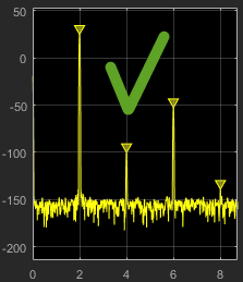
When you set the distortion Type to Intermodulation, the following fields appear in the Intermodulation Distortion panel at the bottom of the spectrum analyzer window.

• F1 — Lower fundamental first-order frequency.

• F2 — Upper fundamental first-order frequency.

• 2F1 - F2 — Lower intermodulation product from third-order harmonics.

• 2F2 - F1 — Upper intermodulation product from third-order harmonics.

• TOI — Third-order intercept point. If the noise power is too high in relation to the harmonics, the TOI value will not be accurate. In this case, you should lower the resolution bandwidth or select a different spectral window. If the TOI has the same amplitude as the input two-tone signal, reduce the power of that input signal.

The intermodulation distortion measurement automatically locates the fundamental and the first-order frequencies (F1 and F2). It then computes the frequencies of the third-order intermodulation products (2F1−F2 and 2F2−F1).

For modifying the distortion measurements programmatically, see the DistortionMeasurementsConfiguration object.

Customize Visualization

Set configuration and style settings in the spectrum analyzer.

To control the settings of the display and labels, color and styling, click Display Settings () on the Home tab of the spectrum analyzer toolstrip.

In the dialog box that opens, you can customize the font size, plot type, y-axis properties of the spectrum plot, and color map properties of the spectrogram plot. You can change the color of the spectrum plot, background, axes, and labels and also change the line properties.

Display Controls

Use the display controls to:

• Zoom and pan the axes.

• Enable and disable the legend and the color bar.

To scale the plot axes, use the mouse to pan around the axes and the scroll button on your mouse to zoom in and out of the plot. Additionally, you can use the buttons that appear when you hover over the plot window.

• — Maximize the axes, hide all labels and inset the axes values.

• — Zoom in on the plot.

• — Pan the plot.

• — Autoscale the axes to fit the shown data.

To enable or disable the legend, click in the spectrum display.

To enable or disable the color bar, click in the spectrogram display.

Tips

If you set the Averaging Method to VBW or Exponential, and you introduce NaN or Inf values into the data, the spectrum appears blank. To ignore the NaN or Inf values:

• In the Home tab > Environment section of the MATLAB toolstrip, click Settings ().

  In the Workspace section of the Settings dialog box, select the Ignore NaNs when calculating statistics check box.

Algorithms

Spectrum Estimation — Welch's Method

When you select the Welch method, the power spectrum estimate is the averaged modified periodograms.

The algorithm in the spectrum analyzer consists of these steps:

1. The block buffers the input into N-point data segments. Each data segment is split into P overlapping data segments, each of length M, overlapping by D points. The data segments can be represented as:

   $$\begin{array}{l}{x}_i(n)=x(n+iD),n=0,1,\mathrm{...},M-1\\ i=0,1,\mathrm{...},P-1\end{array}$$

   • If D = M/2, the overlap is 50%.

   • If D = 0, the overlap is 0%.

2. Apply a window to each of the P overlapping data segments in the time domain.

   The spectrum analyzer uses RBW (Hz) on the Estimation tab to determine the data window length internally.

   Then, it partitions the input signal into a number of windowed data segments.

   Most window functions afford more influence to the data at the center of the set than to the data at the edges, which represents a loss of information. To mitigate that loss, the individual data sets are commonly overlapped in time. For each windowed segment, compute the periodogram by computing the discrete Fourier transform. Then compute the squared magnitude of the result and divide the result by M.

   $$P_{xx}^i(f)=\frac{1}{MU}{\left|{\displaystyle \sum _{n=0}^{M-1}{x}_i(n)w(n)e^{-j2\pi fn}}\right|}^2,i=0,1,\mathrm{...},P-1$$

   where U is the normalization factor for the power in the window function and is given by

   $$U=\frac{1}{M}{\displaystyle \sum _{n=0}^{M-1}{w}^2(n)}$$

   You can specify the window by clicking the Window drop-down arrow on the Estimation tab of the spectrum analyzer toolstrip.

3. The spectrum analyzer calculates and plots the power spectrum, power spectrum density, and RMS using the modified Periodogram estimator. For more information about the Periodogram method, see periodogram (Signal Processing Toolbox).

   To determine the power spectrum estimate for Welch's method, the spectrum analyzer averages the result of the periodograms for the last P data segments. The averaging reduces the variance, compared to the original N-point data segment. For more details on the averaging, see Averaging Method.

   $$\mathrm{PSD}\left(f\right)=\frac{1}{P}{\displaystyle \sum _{i=0}^{P-1}{P}_{xx}^i(f)}$$

   • The spectrum analyzer computes the power spectral density using:

     $$\mathrm{PSD}\left(f\right)=\frac{1}{P*F_s}{\displaystyle \sum _{i=0}^{P-1}{P}_{xx}^i(f)}$$

   • The power spectrum is the product of the power spectral density and the resolution bandwidth, as given by this equation.

     $$P_{spectrum}\left(f\right)=\mathrm{PSD}\left(f\right)\times RBW=\mathrm{PSD}\left(f\right)\times \frac{F_s\times NENBW}{N_{window}}$$

The spectrum analyzer uses a certain number of samples to compute a spectral estimate. This value is directly related to the resolution bandwidth (RBW) using this equation, $$N_{samples}=\frac{\left(1-\frac{O_p}{100}\right)\times NENBW\times F_s}{RBW},$$

where O_p is the overlap percentage, NENBW is the normalized effective noise bandwidth, F_s is the input sample rate, and RBW is the resolution bandwidth.

The spectrum analyzer shows the number of samples per update in the spectrum analyzer status bar. Click the $$⋮$$ icon in the status bar and select Samples/Update (S/U).

The algorithm determines the window length using this equation:

$$N_{window}=\frac{NENBW\times F_s}{RBW}$$

Overlap Percentage (O_p)

The overlap percentage O_p is the value you specify in the Overlap % property. To view the Overlap % parameter, on the Estimation tab on the spectrum analyzer toolstrip, click the Window drop-down arrow.

When you increase the overlap percentage, the spectrum analyzer needs fewer new input samples to compute a new spectral update.

Op	Nsamples
0%	100
50%	50
80%	20

Normalized Effective Noise Bandwidth (NENBW)

The normalized effective noise bandwidth NENBW is a window parameter that measures the noise performance of the window. NENBW is determined using the window length and the window coefficients, and is given by the following equation:

$$NENBW=N_{window}\times \frac{{\displaystyle \sum _{n=1}^{N_{window}}{w}^2(n)}}{{\left[{\displaystyle \sum _{n=1}^{N_{window}}w(n)}\right]}^2},$$

w(n) denotes the vector of window coefficients. N_window is the window length. For more information on how the algorithm determines the window length, see the Spectrum Estimation –– Welch's Method section in Algorithms.

The rectangular window has the smallest NENBW, with a value of 1. All other windows have a larger NENBW value. For example, the Hann window has an NENBW value of approximately 1.5.

The spectrum analyzer shows the value of NENBW in the spectrum analyzer status bar. Click the $$⋮$$ icon in the status bar and select NENBW.

Input Sample Rate (Fs)

F_s is the sample rate of the input signal. You can view the Sample Rate (Hz) on the Home tab of the spectrum analyzer toolstrip. You can enable this property in the status bar at the bottom of the spectrum analyzer window. Click the icon in the status bar and select Sample Rate (Fs).

Resolution Bandwidth (RBW)

Resolution bandwidth controls the spectral resolution of the displayed signal. The RBW value determines the spacing between frequencies that the scope can resolve. A smaller value gives a higher spectral resolution and lowers the noise floor, that is, the spectrum analyzer can resolve frequencies that are closer to each other. However, this comes at the cost of a longer sweep time.

You can specify the resolution bandwidth using the RBW (Hz) parameter.

When you set RBW (Hz) to:

• Auto –– The spectrum analyzer determines the appropriate resolution bandwidth to ensure that there are 1024 RBW intervals over the specified frequency span. When you set RBW (Hz) to Auto, the spectrum analyzer calculates using this equation.

  $$RB{W}_{auto}=\frac{span}{1024}$$

• scalar value –– Specify a value such that there are at least two RBW intervals over the specified frequency span. The ratio of the overall span to RBW must be greater than two:

  $$\frac{span}{RBW}>2$$

span is the frequency span over which the spectrum analyzer computes and plots the spectrum. Spectrum analyzer shows the span through the Span (Hz) property.

When the number of input samples is not sufficient to achieve the specified resolution bandwidth, the spectrum analyzer adjusts its RBW value according to the number of input samples provided and displays a message similar to this one. The spectrum analyzer removes this message once you provide enough input samples.

You can enable this property in the status bar at the bottom of the spectrum analyzer window. Click the icon in the status bar and select RBW.

Nyquist Frequency Interval

When you plot the two-sided spectrum by selecting Two-Sided Spectrum in the Frequency Span options, the Nyquist frequency interval is $$\left[-\frac{SampleRate}{2},\frac{SampleRate}{2}\right]+FrequencyOffset$$ Hz.

When you clear the Two-Sided Spectrum, the Nyquist frequency interval is $$\left[0,\frac{SampleRate}{2}\right]+FrequencyOffset$$ Hz.

Frequency Vector

When you plot the two-sided spectrum by selecting Two-Sided Spectrum in the Frequency Span options, the frequency vector is:

$$\left[-\frac{SampleRate}{2},\frac{SampleRate}{2}\right]$$

When you clear the Two-Sided Spectrum, the frequency vector is:

$$\left[0,\frac{SampleRate}{2}\right]$$

Occupied BW

The spectrum analyzer calculates Occupied BW using these steps.

1. Calculate the total power in the measured frequency range.

2. Determine the lower frequency value. Starting at the lowest frequency in the range and moving upward, sum the power distributed in each frequency until the result is

   $$\frac{100-OccupiedBW\%}{2}$$

   of the total power.

3. Determine the upper frequency value. Starting at the highest frequency in the range and moving downward, sum the power distributed in each frequency until the result reaches

   $$\frac{100-OccupiedBW\%}{2}$$

   of the total power.

4. The bandwidth between the lower and upper power frequency values is the occupied bandwidth.

5. The frequency halfway between the lower and upper frequency values is the center frequency.

Distortion Measurements

The spectrum analyzer calculates Distortion Measurements using these steps.

1. Estimate spectral content by finding peaks in the spectrum. When the algorithm detects a peak, it records the width of the peak and clears all monotonically decreasing values by treating all these values as if they belong to the peak. Using this method, the algorithm removes all spectral content centered at DC (0 Hz) from the spectrum and records the amount of bandwidth cleared (W₀).

2. Determine the fundamental power (P₁) from the remaining maximum value of the displayed spectrum. Create a local estimate (Fe₁) of the fundamental frequency by computing the central moment of the power near the peak. Record the bandwidth of the fundamental power content (W₁). Then remove the power from the fundamental as in step 1.

3. Determine the power and width of the higher-order harmonics (P₂, W₂, P₃, W₃, etc.) in succession by examining the frequencies closest to the appropriate multiple of the local estimate (Fe₁). Remove any spectral content that decreases monotonically about the harmonic frequency from the spectrum before proceeding to the next harmonic.

4. After removing the DC, fundamental, and harmonic content from the spectrum, examine the power of the remaining spectrum for its sum (P_remaining), peak value (P_maxspur), and median value (P_estnoise).

5. Compute the sum of all the removed bandwidth as W_sum = W₀ + W₁ + W₂ +...+ W_n.

   Compute the sum of powers of the second and higher-order harmonics as P_harmonic = P₂ + P₃ + P₄ +...+ P_n.

6. Estimate the sum of the noise power as:

   $$P_{noise}=(P_{remaining}\cdot dF+P_{est.noise}\cdot W_{sum})/RBW$$

   Where dF is the absolute difference between frequency bins, and RBW is the resolution bandwidth of the window.

7. Then compute the metrics for THD, THD%, SINAD, SNR, and SFDR from the estimates.

   $$\begin{array}{l}THD=10\cdot {\log }_{10}\left(\frac{P_{harmonic}}{P_1}\right)\\ THD\%=100\cdot {10}^{\left(THD/20\right)}\\ SINAD=10\cdot {\log }_{10}\left(\frac{P_1}{P_{harmonic}+P_{noise}}\right)\\ SNR=10\cdot {\log }_{10}\left(\frac{P_1}{P_{noise}}\right)\\ SFDR=10\cdot {\log }_{10}\left(\frac{P_1}{\max \left(P_{maxspur},\max \left(P_2,P_3,\mathrm{...},P_n\right)\right)}\right)\end{array}$$

Harmonic Measurements

1. The harmonic distortion measurements use the spectrum trace shown in the display as the input to the measurements. The default Hann window setting of the spectrum analyzer might exhibit leakage that can completely mask the noise floor of the measured signal.

   The harmonic measurements attempt to correct for leakage by ignoring all frequency content that decreases monotonically away from the maximum of harmonic peaks. If the window leakage covers more than 70% of the frequency bandwidth in your spectrum, you may see a blank reading (–) reported for SNR and SINAD. If your application can tolerate the increased equivalent noise bandwidth (ENBW), consider using a Kaiser window with a high attenuation (up to 300 dB) to minimize spectral leakage.

2. Ignore the DC component.

3. After windowing, the width of each harmonic component masks the noise power in the neighborhood of the fundamental frequency and harmonics. To estimate the noise power in each region, the spectrum analyzer computes the median noise level in the nonharmonic areas of the spectrum. It then extrapolates that value into each region.

4. N^th order intermodulation products occur at A*F1 + B*F2,

   where F1 and F2 are the sinusoid input frequencies and |A| + |B| = N. A and B are integer values.

5. For intermodulation measurements, compute the third-order intercept (TOI) point as follows.

   • TOI_lower = P_F1 + (P_F2 - P_(2F1-F2))/2

   • TOI_upper = P_F2 + (P_F1 - P_(2F2-F1))/2

   • TOI = (TOI_lower + TOI_upper)/2

   Where P is power in decibels of the measured power referenced to 1 milliwatt (dBm).

Averaging Method

The spectrum analyzer calculates the moving average using one of these methods:

• Video bandwidth — The spectrum analyzer uses a time-domain lowpass filter to smooth the noise in the signal. The video bandwidth (VBW) filter smoothes the trace and decreases noise, and the spectrum analyzer applies the filter to the data before displaying it.

  Video bandwidth is the bandwidth of the lowpass filter that spectrum analyzer uses to average or smooth the noise in the signal before displaying it in the scope. The spectrum analyzer computes the video bandwidth using this equation:

  $$VBW=\frac{(1-\lambda )RBW}{2\pi \lambda NENBW}$$

  where,

  • λ is the forgetting factor.

  • RBW is the resolution bandwidth.

  • NENBW is the normalized effective noise bandwidth.

  Video bandwidth does not affect the level of the noise (noise floor), but only increases the signal-to-noise ratio and smoothes the trace of the noise. When you decrease the value of VBW, the signal-to-noise ratio improves.

  The cutoff frequency of the video bandwidth filter is given by:

  $${\omega }_c=\frac{2\pi VBW}{F_s/NFFT}$$

  where Fs is the input sample rate and NFFT is the number of FFT points.

  The spectrum analyzer shows the values of sample rate, VBW, and NFFT in the status bar at the bottom of the display. To enable, right-click the status bar and select Sample Rate (Fs), VBW, and FFT Length (NFFT).

• Exponential — The moving average algorithm uses the exponential weighting method to update the weights and compute the moving average recursively for each Z vector that comes in by using the following recursive equations:

  $$\begin{array}{l}{w}_N=\lambda w_{N-1}+1\\ {\overline{z}}_N=\left(1-\frac{1}{w_N}\right){\overline{z}}_{N-1}+\left(\frac{1}{w_N}\right)z_N\end{array}$$

  • λ — Forgetting factor

  • $$w_N$$ — Weighting factor applied to the current Z vector

  • $$z_N$$ — Current Z vector

  • $${\overline{z}}_{N-1}$$ — Moving average until the previous Z vector

  • $$\left(1-\frac{1}{w_N}\right){\overline{z}}_{N-1}$$ — Effect of the previous Z vectors on the average

  • $${\overline{z}}_N$$ — Moving average including the current Z vector

• Running –– For each frame of the input, average the last Q scaled Z vectors, which are computed by the algorithm. The variable Q is the value you specify for the number of spectral averages. If the algorithm does not have enough Z vectors, the algorithm uses zeros to fill the empty elements.

Extended Capabilities

C/C++ Code Generation

Generate C and C++ code using Simulink® Coder™.

This block can be used for simulation visibility in systems that generate code. However, the block is not included in the generated code.

Version History

Introduced in R2017b

R2026b: New streamlined user interface in spectrum analyzer

The spectrum analyzer toolstrip has been reorganized into these three tabs to give you an easy and streamlined access to the scope settings.

• Home tab contains all the general settings for the spectrum display.

• Estimation tab contains settings that control the frequency resolution and spectral averaging.

• Measurements tab contains settings to control the various measurements supported by the scope.

R2026b: Updated status bar readouts

Certain parameter names in the spectrum analyzer status bar have changed. Some of these parameters have new readouts. For more information, see the following table.

Status Bar Parameter In R2026a or Earlier	Status Bar Parameter In R2026b	Status Bar Readout In R2026b
Sample Rate	Sample Rate (Fs)	Fs
Samples/Update	Samples/Update (S/U)	S/U
Time Resolution	Time Resolution (ΔT)	ΔT
NFFT	FFT Length (NFFT)	NFFT
Forgetting Factor	Forgetting Factor (α)	α
Spectral Averages	Spectral Averages (Navg)	Navg

R2026a: Autoscaling of y-axis limits

You can now automatically scale the y-axis limits of the spectrum analyzer display by selecting the Automatically Scale Axes Limits parameter. If you clear this parameter, the Y-Limits parameter enables you to manually scale the axes limits.

R2025a: Control plot type for each line individually

You can now individually control the type of plot for each line. To control the type of plot for a line, select the line and set the Plot Type parameter accordingly.

R2025a: Support for running averaging method

The Spectrum Analyzer block now supports the running averaging method to compute the power spectrum estimate. To enable this mode, set the Averaging Method parameter in the Estimation tab to Running and the Spectral Averages parameter to a positive integer.

For more information, see the Algorithms section.

R2024b: Display spectral data for any number of input samples and adjust RBW accordingly

Previously, the Spectrum Analyzer block required a minimum number of samples to update the display for a given RBW value. Starting in R2024b, this limitation is removed. The scope now updates its display for any number of input samples and adjusts the RBW value accordingly.

R2024b: Auto adjust RBW to maintain 1024 samples

The Spectrum Analyzer block can now automatically adjust the resolution bandwidth (RBW) so as to maintain the number of samples per spectral update at 1024 (Nsamples = 1024) irrespective of the window you select.

To enable this mode in the Spectrum Analyzer block, set:

• RBW (Hz) to Auto.

R2024b: Higher display precision in scope UI

You can now increase the display precision to 15 digits using the Display Precision property in the scope settings under Display and Labels. This precision affects all the measurements and data that the scope displays on its status bar.

R2024b: Preserve Colors is now available in scope toolstrip

The Preserve colors for copy to clipboard property has been renamed to Preserve Colors and is now available in the scope toolstrip under Copy Display.

R2024a: Analyzer tab has been renamed as Scope tab

The Analyzer tab in spectrum analyzer has been renamed as Scope tab.

R2023b: Spectrum Analyzer supports dBuV units

You can set Spectrum Unit to dBuV when you set Spectrum to RMS.

R2023a: Spectrum Analyzer with improved responsiveness and toolstrip interface in Simulink

In R2023a, the Spectrum Analyzer block is more responsive and its toolstrip interface is improved to provide you easy access to spectral analysis, estimation, and measurements. You can configure and display Spectrum Analyzer settings from the command line with the SpectrumAnalyzerBlockConfiguration object.