spectrogram

Spectrogram using short-time Fourier transform

Syntax

s = spectrogram(x)

[s,f,t] = spectrogram(x,win,nOverlap,freqSpec)

[s,f,t] = spectrogram(x,win,nOverlap,freqSpec,Fs)

[___,ps] = spectrogram(___,freqRange,spectrumType)

[___,fc,tc] = spectrogram(___,"reassigned")

[___] = spectrogram(___,"yaxis",Name=Value)

spectrogram(___)

Description

The spectrogram of a signal is the magnitude squared of its Short-Time Fourier Transform (STFT). The STFT describes how the frequency content of a signal changes over time.

s = spectrogram(x) returns the STFT of the signal x. Each column of s contains an estimate of the short-term, time-localized frequency content of x.

[s,f,t] = spectrogram(x,win,nOverlap,freqSpec) returns the STFT of the signal x and the frequencies f (rad/sample) and sample indices t, where the spectrogram function:

• Uses win to divide the signal into segments and windows them.

• Uses the overlap length specified in nOverlap to overlap samples between adjoining segments.

• Computes the discrete Fourier transform of each windowed segment over the number of points or at the frequencies specified in freqSpec.

To use default values for any of these input arguments, specify them as empty, [].

[s,f,t] = spectrogram(x,win,nOverlap,freqSpec,Fs) specifies the sample rate Fs and returns the cyclical frequencies f (Hz) and time instants t.

[___,ps] = spectrogram(___,freqRange,spectrumType) also specifies the frequency range and spectrum type to return in ps, which is proportional to the spectrogram of x. Return ps either as a power spectral density (PSD) estimate or as a power spectrum estimate. You can specify either or both of these input arguments.

[___,fc,tc] = spectrogram(___,"reassigned") reassigns each PSD estimate or power spectrum estimate to the location of its center of energy. This syntax also returns the center-of-energy frequencies and times, fc and tc.

If your signal contains well-localized temporal or spectral components, then the "reassigned" argument generates a sharper spectrogram.

[___] = spectrogram(___,"yaxis",Name=Value) specifies additional options using name-value arguments. You can specify the minimum threshold, the output time dimension, and the target parent container on which to plot the spectrogram.

If you specify a target parent container, then the "yaxis" option displays the frequency on the y-axis and the time on the x-axis in the plot of ps.

spectrogram(___) with no output arguments plots ps in decibels in the current figure window or specified target parent container.

Examples

Default Values of Spectrogram

Generate $$N_x=1024$$ samples of a signal that consists of a sum of sinusoids. The normalized frequencies of the sinusoids are $$2\pi /5$$ rad/sample and $$4\pi /5$$ rad/sample. The higher frequency sinusoid has 10 times the amplitude of the other sinusoid.

N = 1024;
n = 0:N-1;

w0 = 2*pi/5;
x = sin(w0*n)+10*sin(2*w0*n);

Compute the short-time Fourier transform using the function defaults. Plot the spectrogram.

s = spectrogram(x);

spectrogram(x,"yaxis")

Repeat the computation.

• Divide the signal into sections of length $$nsc=\lfloor N_x/4.5\rfloor$$.

• Window the sections using a Hamming window.

• Specify 50% overlap between contiguous sections.

• To compute the FFT, use $$\max (256,2^p)$$ points, where $$p=\lceil {\log }_{2}nsc\rceil$$.

Verify that the two approaches give identical results.

Nx = length(x);
nsc = floor(Nx/4.5);
nov = floor(nsc/2);
nff = max(256,2^nextpow2(nsc));

t = spectrogram(x,hamming(nsc),nov,nff);

maxerr = max(abs(abs(t(:))-abs(s(:))))

maxerr = 
0

Divide the signal into 8 sections of equal length, with 50% overlap between sections. Specify the same FFT length as in the preceding step. Compute the short-time Fourier transform and verify that it gives the same result as the previous two procedures.

ns = 8;
ov = 0.5;
lsc = floor(Nx/(ns-(ns-1)*ov));

t = spectrogram(x,lsc,floor(ov*lsc),nff);

maxerr = max(abs(abs(t(:))-abs(s(:))))

maxerr = 
0

Compare spectrogram Function and STFT Definition

Generate a signal that consists of a complex-valued convex quadratic chirp sampled at 600 Hz for 2 seconds. The chirp has an initial frequency of 250 Hz and a final frequency of 50 Hz.

fs = 6e2;
ts = 0:1/fs:2;
x = chirp(ts,250,ts(end),50,"quadratic",0,"convex","complex");

spectrogram Function

Use the spectrogram function to compute the STFT of the signal.

• Divide the signal into segments, each $M=49$ samples long.

• Specify $L=11$ samples of overlap between adjoining segments.

• Discard the final, shorter segment.

• Window each segment with a Bartlett window.

• Evaluate the discrete Fourier transform of each segment at $N_{\text{DFT}}=1024$ points. By default, spectrogram computes two-sided transforms for complex-valued signals.

M = 49;
L = 11;
g = bartlett(M);
Ndft = 1024;

[s,f,t] = spectrogram(x,g,L,Ndft,fs);

Use the waterplot function to compute and display the spectrogram, defined as the magnitude squared of the STFT.

waterplot(s,f,t)

STFT Definition

Compute the STFT of the $N_x$-sample signal using the definition. Divide the signal into $$\lfloor \frac{N_x-L}{M-L}\rfloor$$ overlapping segments. Window each segment and evaluate its discrete Fourier transform at $N_{\text{DFT}}$ points.

segs = framesig(1:length(x),M,OverlapLength=L);
X = fft(x(segs).*g,Ndft);

Compute the time and frequency ranges for the STFT.

• To find the time values, divide the time vector into overlapping segments. The time values are the midpoints of the segments, with each segment treated as an interval open at the lower end.

• To find the frequency values, specify a Nyquist interval closed at zero frequency and open at the lower end.

framedT = ts(segs);
tint = mean(framedT(2:end,:));

fint = 0:fs/Ndft:fs-fs/Ndft;

Compare the output of spectrogram to the definition. Display the spectrogram.

maxdiff = max(max(abs(s-X)))

maxdiff = 
0

waterplot(X,fint,tint)

function waterplot(s,f,t)
% Waterfall plot of spectrogram
    waterfall(f,t,abs(s)'.^2)
    set(gca,XDir="reverse",View=[30 50])
    xlabel("Frequency (Hz)")
    ylabel("Time (s)")
end

Compare spectrogram and stft Functions

Generate a signal consisting of a chirp sampled at 1.4 kHz for 2 seconds. The frequency of the chirp decreases linearly from 600 Hz to 100 Hz during the measurement time.

fs = 1400;
x = chirp(0:1/fs:2,600,2,100);

stft Defaults

Compute the STFT of the signal using the spectrogram and stft functions. Use the default values of the stft function:

• Divide the signal into 128-sample segments and window each segment with a periodic Hann window.

• Specify 96 samples of overlap between adjoining segments. This length is equivalent to 75% of the window length.

• Specify 128 DFT points and center the STFT at zero frequency, with the frequency expressed in hertz.

Verify that the two results are equal.

M = 128;
g = hann(M,"periodic");
L = 0.75*M;
Ndft = 128;

[sp,fp,tp] = spectrogram(x,g,L,Ndft,fs,"centered");

[s,f,t] = stft(x,fs);

dff = max(max(abs(sp-s)))

dff = 
0

Use the mesh function to plot the two outputs.

nexttile
mesh(tp,fp,abs(sp).^2)
title("spectrogram")
view(2), axis tight

nexttile
mesh(t,f,abs(s).^2)
title("stft")
view(2), axis tight

spectrogram Defaults

Repeat the computation using the default values of the spectrogram function:

• Divide the signal into segments of length $M=\lfloor N_x/4.5\rfloor$, where $N_x$ is the length of the signal. Window each segment with a Hamming window.

• Specify 50% overlap between segments.

• To compute the FFT, use $\max \left(256,2^{\lceil {\log }_{2}M\rceil }\right)$ points. Compute the spectrogram only for positive normalized frequencies.

M = floor(length(x)/4.5);
g = hamming(M);
L = floor(M/2);
Ndft = max(256,2^nextpow2(M));

[sx,fx,tx] = spectrogram(x);

[st,ft,tt] = stft(x,Window=g,OverlapLength=L, ...
    FFTLength=Ndft,FrequencyRange="onesided");

dff = max(max(sx-st))

dff = 
0

Use the waterplot function to plot the two outputs. Divide the frequency axis by $\pi$ in both cases. For the stft output, divide the sample numbers by the effective sample rate, $2\pi$.

figure
nexttile
waterplot(sx,fx/pi,tx)
title("spectrogram")

nexttile
waterplot(st,ft/pi,tt/(2*pi))
title("stft")

function waterplot(s,f,t)
% Waterfall plot of spectrogram
    waterfall(f,t,abs(s)'.^2)
    set(gca,XDir="reverse",View=[30 50])
    xlabel("Frequency/\pi")
    ylabel("Samples")
end

Spectrogram and Instantaneous Frequency

Use the spectrogram function to measure and track the instantaneous frequency of a signal.

Generate a quadratic chirp sampled at 1 kHz for two seconds. Specify the chirp so that its frequency is initially 100 Hz and increases to 200 Hz after one second.

fs = 1000;
t = 0:1/fs:2-1/fs;
y = chirp(t,100,1,200,"quadratic");

Estimate the spectrum of the chirp using the short-time Fourier transform implemented in the spectrogram function. Divide the signal into sections of length 100, windowed with a Hamming window. Specify 80 samples of overlap between adjoining sections and evaluate the spectrum at $$\lfloor 100/2+1\rfloor =51$$ frequencies.

spectrogram(y,100,80,100,fs,"yaxis")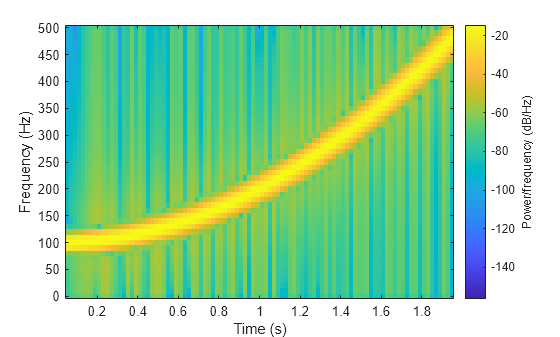

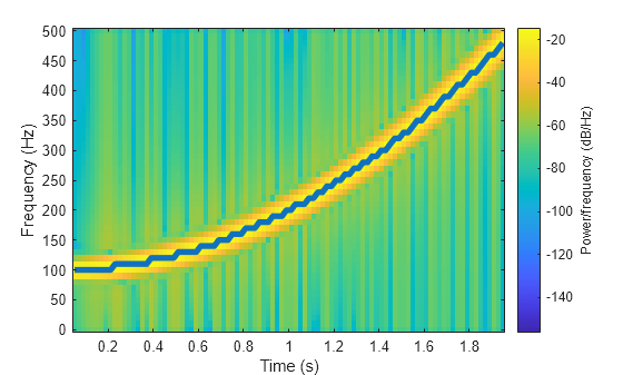
Track the chirp frequency by finding the time-frequency ridge with highest energy across the $$\lfloor (2000-80)/(100-80)\rfloor =96$$ time points. Overlay the instantaneous frequency on the spectrogram plot.

[~,f,t,p] = spectrogram(y,100,80,100,fs);

[fridge,~,lr] = tfridge(p,f);

hold on
plot3(t,fridge,abs(p(lr)),LineWidth=2)
hold off

Spectrogram of Complex Signal

Generate 512 samples of a chirp with sinusoidally varying frequency content.

N = 512;
n = 0:N-1;

x = exp(1j*pi*sin(8*n/N)*32);

Compute the centered two-sided short-time Fourier transform of the chirp. Divide the signal into 32-sample segments with 16-sample overlap. Specify 64 DFT points. Plot the spectrogram.

[scalar,fs,ts] = spectrogram(x,32,16,64,"centered");

spectrogram(x,32,16,64,"centered","yaxis")

Obtain the same result by computing the spectrogram on 64 equispaced frequencies over the interval $\left(-\pi ,\pi \right]$. The 'centered' option is not necessary.

fintv = -pi+pi/32:pi/32:pi;

[vector,fv,tv] = spectrogram(x,32,16,fintv);

spectrogram(x,32,16,fintv,"yaxis")

Compare spectrogram and pspectrum Functions

Generate a signal that consists of a voltage-controlled oscillator and three Gaussian atoms. The signal is sampled at $f_s=2$ kHz for 2 seconds.

fs = 2000;
tx = 0:1/fs:2;
gaussFun = @(A,x,mu,f) exp(-(x-mu).^2/(2*0.03^2)).*sin(2*pi*f.*x)*A';
s = gaussFun([1 1 1],tx',[0.1 0.65 1],[2 6 2]*100)*1.5;
x = vco(chirp(tx+.1,0,tx(end),3).*exp(-2*(tx-1).^2),[0.1 0.4]*fs,fs);
x = s+x';

Short-Time Fourier Transforms

Use the pspectrum function to compute the STFT.

• Divide the $N_x$-sample signal into segments of length $M=80$ samples, corresponding to a time resolution of $80/2000=40$ milliseconds.

• Specify $L=16$ samples or 20% of overlap between adjoining segments.

• Window each segment with a Kaiser window and specify a leakage $\ell =0.7$.

M = 80;
L = 16;
lk = 0.7;

[S,F,T] = pspectrum(x,fs,"spectrogram", ...
    TimeResolution=M/fs,OverlapPercent=L/M*100, ...
    Leakage=lk);

Compare to the result obtained with the spectrogram function.

• Specify the window length and overlap directly in samples.

• pspectrum always uses a Kaiser window as $g\left(n\right)$. The leakage $\ell$ and the shape factor $\beta$ of the window are related by $\beta =40\times \left(1-\ell \right)$.

• pspectrum always uses $N_{\text{DFT}}=1024$ points when computing the discrete Fourier transform. You can specify this number if you want to compute the transform over a two-sided or centered frequency range. However, for one-sided transforms, which are the default for real signals, spectrogram uses $1024/2+1=513$ points. Alternatively, you can specify the vector of frequencies at which you want to compute the transform, as in this example.

• If a signal cannot be divided exactly into $k=\lfloor \frac{N_x-L}{M-L}\rfloor$ segments, spectrogram truncates the signal whereas pspectrum pads the signal with zeros to create an extra segment. To make the outputs equivalent, remove the final segment and the final element of the time vector.

• spectrogram returns the STFT, whose magnitude squared is the spectrogram. pspectrum returns the segment-by-segment power spectrum, which is already squared but is divided by a factor of $\sum _{n}g\left(n\right)$ before squaring.

• For one-sided transforms, pspectrum adds an extra factor of 2 to the spectrogram.

g = kaiser(M,40*(1-lk));

k = (length(x)-L)/(M-L);
if k~=floor(k)
    S = S(:,1:floor(k));
    T = T(1:floor(k));
end

[s,f,t] = spectrogram(x/sum(g)*sqrt(2),g,L,F,fs);

Use the waterplot function to display the spectrograms computed by the two functions.

subplot(2,1,1)
waterplot(sqrt(S),F,T)
title("pspectrum")

subplot(2,1,2)
waterplot(s,f,t)
title("spectrogram")

maxd = max(max(abs(abs(s).^2-S)))

maxd = 
2.4419e-08

Power Spectra and Convenience Plots

The spectrogram function has a fourth argument that corresponds to the segment-by-segment power spectrum or power spectral density. Similar to the output of pspectrum, the ps argument is already squared and includes the normalization factor $\sum _{n}g\left(n\right)$. For one-sided spectrograms of real signals, you still have to include the extra factor of 2. Set the scaling argument of the function to "power".

[~,~,~,ps] = spectrogram(x*sqrt(2),g,L,F,fs,"power");

max(abs(S(:)-ps(:)))

ans = 
2.4419e-08

When called with no output arguments, both pspectrum and spectrogram plot the spectrogram of the signal in decibels. Include the factor of 2 for one-sided spectrograms. Set the colormaps to be the same for both plots. Set the x-limits to the same values to make visible the extra segment at the end of the pspectrum plot. In the spectrogram plot, display the frequency on the y-axis.

subplot(2,1,1)
pspectrum(x,fs,"spectrogram", ...
    TimeResolution=M/fs,OverlapPercent=L/M*100, ...
    Leakage=lk)
title("pspectrum")
cc = clim;
xl = xlim;

subplot(2,1,2)
spectrogram(x*sqrt(2),g,L,F,fs,"power","yaxis")
title("spectrogram")
clim(cc)
xlim(xl)

function waterplot(s,f,t)
% Waterfall plot of spectrogram
    waterfall(f,t,abs(s)'.^2)
    set(gca,XDir="reverse",View=[30 50])
    xlabel("Frequency (Hz)")
    ylabel("Time (s)")
end

Reassigned Spectrogram of Quadratic Chirp

Generate a chirp signal sampled for 2 seconds at 1 kHz. Specify the chirp so that its frequency is initially 100 Hz and increases to 200 Hz after 1 second.

fs = 1000;
t = 0:1/fs:2;
y = chirp(t,100,1,200,"quadratic");

Estimate the reassigned spectrogram of the signal.

• Divide the signal into sections of length 128, windowed with a Kaiser window with shape parameter $$\beta =18$$.

• Specify 120 samples of overlap between adjoining sections.

• Evaluate the spectrum at $$\lfloor 128/2\rfloor =65$$ frequencies and $$\lfloor (length(x)-120)/(128-120)\rfloor =235$$ time bins.

Use the spectrogram function with no output arguments to plot the reassigned spectrogram. Display frequency on the y-axis and time on the x-axis.

spectrogram(y,kaiser(128,18),120,128,fs,"reassigned","yaxis")

Redo the plot using the imagesc function. Specify the y-axis direction so that the frequency values increase from bottom to top. Add eps to the reassigned spectrogram to avoid potential negative infinities when converting to decibels.

[~,fr,tr,pxx] = spectrogram(y,kaiser(128,18),120,128,fs,"reassigned");

imagesc(tr,fr,pow2db(pxx+eps))
axis xy
xlabel("Time (s)")
ylabel("Frequency (Hz)")
colorbar

Spectrogram with Threshold

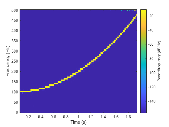
Generate a chirp signal sampled for 2 seconds at 1 kHz. Specify the chirp so that its frequency is initially 100 Hz and increases to 200 Hz after 1 second.

Fs = 1000;
t = 0:1/Fs:2;
y = chirp(t,100,1,200,"quadratic");

Estimate the time-dependent power spectral density (PSD) of the signal.

• Divide the signal into sections of length 128, windowed with a Kaiser window with shape parameter $$\beta =18$$.

• Specify 120 samples of overlap between adjoining sections.

• Evaluate the spectrum at $$\lfloor 128/2\rfloor =65$$ frequencies and $$\lfloor (length(x)-120)/(128-120)\rfloor =235$$ time bins.

Output the frequency and time of the center of gravity of each PSD estimate. Set to zero those elements of the PSD smaller than $$-30$$ dB.

[~,~,~,pxx,fc,tc] = spectrogram(y,kaiser(128,18),120,128,Fs, ...
    MinThreshold=-30);

Plot the nonzero elements as functions of the center-of-gravity frequencies and times.

plot(tc(pxx>0),fc(pxx>0),".")

Compute Centered and One-Sided Spectrograms

Generate a signal that consists of a real-valued chirp sampled at 2 kHz for 2 seconds.

fs = 2000;
tx = 0:1/fs:2;
x = vco(-chirp(tx,0,tx(end),2).*exp(-3*(tx-1).^2), ...
    [0.1 0.4]*fs,fs).*hann(length(tx))';

Two-Sided Spectrogram

Compute and plot the two-sided STFT of the signal.

• Divide the signal into segments, each $M=73$ samples long.

• Specify $L=24$ samples of overlap between adjoining segments.

• Discard the final, shorter segment.

• Window each segment with a flat-top window.

• Evaluate the discrete Fourier transform of each segment at $N_{\text{DFT}}=895$ points, noting that it is an odd number.

M = 73;
L = 24;
g = flattopwin(M);
Ndft = 895;
neven = ~mod(Ndft,2);

[stwo,f,t] = spectrogram(x,g,L,Ndft,fs,"twosided");

Use the spectrogram function with no output arguments to plot the two-sided spectrogram.

spectrogram(x,g,L,Ndft,fs,"twosided","power","yaxis")

Compute the two-sided spectrogram using the definition. Divide the signal into $M$-sample segments with $L$ samples of overlap between adjoining segments. Window each segment and compute its discrete Fourier transform at $N_{\text{DFT}}$ points.

y = framesig(x,M,Window=g,OverlapLength=L);
Xtwo = fft(y,Ndft);

Compute the time and frequency ranges.

• To find the time values, divide the time vector into overlapping segments. The time values are the midpoints of the segments, with each segment treated as an interval open at the lower end.

• To find the frequency values, specify a Nyquist interval closed at zero frequency and open at the upper end.

framedT = framesig(tx,M,OverlapLength=L);
ttwo = mean(framedT(2:end,:));

ftwo = 0:fs/Ndft:fs*(1-1/Ndft);

Compare the outputs of spectrogram to the definitions. Use the waterplot function to display the spectrograms.

diffs = [max(max(abs(stwo-Xtwo)));
    max(abs(f-ftwo'));
    max(abs(t-ttwo))]

diffs = 3×1
10-12 ×

         0
    0.2274
    0.0002

figure
nexttile
waterplot(Xtwo,ftwo,ttwo)
title("Two-Sided, Definition")

nexttile
waterplot(stwo,f,t)
title("Two-Sided, spectrogram Function")

Centered Spectrogram

Compute the centered spectrogram of the signal.

• Use the same time values that you used for the two-sided STFT.

• Use the fftshift function to shift the zero-frequency component of the STFT to the center of the spectrum.

• For odd-valued $N_{\text{DFT}}$, the frequency interval is open at both ends. For even-valued $N_{\text{DFT}}$, the frequency interval is open at the lower end and closed at the upper end.

Compare the outputs and display the spectrograms.

tcen = ttwo;

if ~neven
    Xcen = fftshift(Xtwo,1);
    fcen = -fs/2*(1-1/Ndft):fs/Ndft:fs/2;
else
    Xcen = fftshift(circshift(Xtwo,-1),1);
    fcen = (-fs/2*(1-1/Ndft):fs/Ndft:fs/2)+fs/Ndft/2;
end

[scen,f,t] = spectrogram(x,g,L,Ndft,fs,"centered");

diffs = [max(max(abs(scen-Xcen)));
    max(abs(f-fcen'));
    max(abs(t-tcen))]

diffs = 3×1
10-12 ×

         0
    0.2274
    0.0002

figure
nexttile
waterplot(Xcen,fcen,tcen)
title("Centered, Definition")

nexttile
waterplot(scen,f,t)
title("Centered, spectrogram Function")

One-Sided Spectrogram

Compute the one-sided spectrogram of the signal.

• Use the same time values that you used for the two-sided STFT.

• For odd-valued $N_{\text{DFT}}$, the one-sided STFT consists of the first $\left(N_{\text{DFT}}+1\right)/2$ rows of the two-sided STFT. For even-valued $N_{\text{DFT}}$, the one-sided STFT consists of the first $N_{\text{DFT}}/2+1$ rows of the two-sided STFT.

• For odd-valued $N_{\text{DFT}}$, the frequency interval is closed at zero frequency and open at the Nyquist frequency. For even-valued $N_{\text{DFT}}$, the frequency interval is closed at both ends.

Compare the outputs and display the spectrograms. For real-valued signals, the "onesided" argument is optional.

tone = ttwo;

if ~neven
    Xone = Xtwo(1:(Ndft+1)/2,:);
else
    Xone = Xtwo(1:Ndft/2+1,:);
end

fone = 0:fs/Ndft:fs/2;

[sone,f,t] = spectrogram(x,g,L,Ndft,fs);

diffs = [max(max(abs(sone-Xone)));
    max(abs(f-fone'));
    max(abs(t-tone))]

diffs = 3×1
10-12 ×

         0
    0.1137
    0.0002

figure
nexttile
waterplot(Xone,fone,tone)
title("One-Sided, Definition")

nexttile
waterplot(sone,f,t)
title("One-Sided, spectrogram Function")

function waterplot(s,f,t)
% Waterfall plot of spectrogram
waterfall(f,t,abs(s)'.^2)
set(gca,XDir="reverse",View=[30 50])
xlabel("Frequency (Hz)")
ylabel("Time (s)")
end

Compute Segment PSDs and Power Spectra

The spectrogram function has a matrix containing either the power spectral density (PSD) or the power spectrum of each segment as the fourth output argument. The power spectrum is equal to the PSD multiplied by the equivalent noise bandwidth (ENBW) of the window.

Generate a signal that consists of a logarithmic chirp sampled at 1 kHz for 1 second. The chirp has an initial frequency of 400 Hz that decreases to 10 Hz by the end of the measurement.

fs = 1000;
tt = 0:1/fs:1-1/fs;
y = chirp(tt,400,tt(end),10,"logarithmic");

Segment PSDs and Power Spectra with Sample Rate

Divide the signal into 102-sample segments and window each segment with a Hann window. Specify 12 samples of overlap between adjoining segments and 1024 DFT points.

M = 102;
g = hann(M);
L = 12;
Ndft = 1024;

Compute the spectrogram of the signal with the default PSD spectrum type. Output the STFT and the array of segment power spectral densities.

[s,f,t,p] = spectrogram(y,g,L,Ndft,fs);

Repeat the computation with the spectrum type specified as "power". Output the STFT and the array of segment power spectra.

[r,~,~,q] = spectrogram(y,g,L,Ndft,fs,"power");

Verify that the spectrogram is the same in both cases. Plot the spectrogram using a logarithmic scale for the frequency.

max(max(abs(s).^2-abs(r).^2))

ans = 
0

waterfall(f,t,abs(s)'.^2)
set(gca,XScale="log",...
    XDir="reverse",View=[30 50])

Verify that the power spectra are equal to the power spectral densities multiplied by the ENBW of the window.

max(max(abs(q-p*enbw(g,fs))))

ans = 
1.6653e-16

Verify that the matrix of segment power spectra is proportional to the spectrogram. The proportionality factor is the square of the sum of the window elements.

max(max(abs(s).^2-q*sum(g)^2))

ans = 
1.3235e-23

Segment PSDs and Power Spectra with Normalized Frequencies

Repeat the computation, but now work in normalized frequencies. The results are the same when you specify the sample rate as $2\pi$.

[~,~,~,pn] = spectrogram(y,g,L,Ndft);
[~,~,~,qn] = spectrogram(y,g,L,Ndft,"power");

max(max(abs(qn-pn*enbw(g,2*pi))))

ans = 
1.1102e-16

Track Chirps in Audio Signal

Load an audio signal that contains two decreasing chirps and a wideband splatter sound. Compute the short-time Fourier transform. Divide the waveform into 400-sample segments with 300-sample overlap. Plot the spectrogram.

load splat

% To hear, type soundsc(y,Fs)

sg = 400;
ov = 300;

spectrogram(y,sg,ov,[],Fs,"yaxis")
colormap bone

Use the spectrogram function to output the power spectral density (PSD) of the signal.

[s,f,t,p] = spectrogram(y,sg,ov,[],Fs);

Track the two chirps using the medfreq function. To find the stronger, low-frequency chirp, restrict the search to frequencies above 100 Hz and to times before the start of the wideband sound.

f1 = f > 100;
t1 = t < 0.75;

m1 = medfreq(p(f1,t1),f(f1));

To find the faint high-frequency chirp, restrict the search to frequencies above 2500 Hz and to times between 0.3 seconds and 0.65 seconds.

f2 = f > 2500;
t2 = t > 0.3 & t < 0.65;

m2 = medfreq(p(f2,t2),f(f2));

Overlay the result on the spectrogram. Divide the frequency values by 1000 to express them in kHz.

hold on
plot(t(t1),m1/1000,LineWidth=4)
plot(t(t2),m2/1000,LineWidth=4)
hold off

3D Spectrogram Visualization

Generate two seconds of a signal sampled at 10 kHz. Specify the instantaneous frequency of the signal as a triangular function of time.

fs = 10e3;
t = 0:1/fs:2;
x1 = vco(sawtooth(2*pi*t,0.5),[0.1 0.4]*fs,fs);

Compute and plot the spectrogram of the signal. Use a Kaiser window of length 256 and shape parameter $$\beta =5$$. Specify 220 samples of section-to-section overlap and 512 DFT points. Plot the frequency on the y-axis. Use the default colormap and view.

spectrogram(x1,kaiser(256,5),220,512,fs,"yaxis")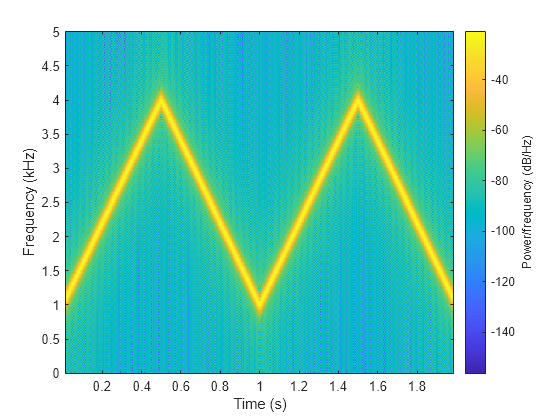

Change the view to display the spectrogram as a waterfall plot. Set the colormap to bone.

view(-45,65)
colormap bone

Plot Spectrogram in Target Axes and Panel Container

Since R2025a

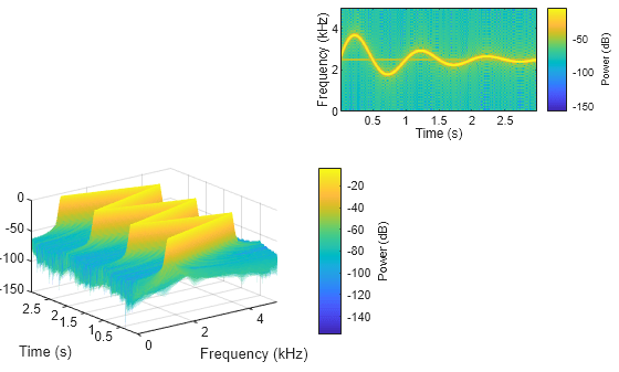
Plot the spectrograms for four signals in the specified target axes and panel containers.

Create four oscillating signals with a sample rate of 10 kHz for three seconds.

Fs = 10e3;
t = 0:1/Fs:3;
x1 = vco(sawtooth(2*pi*t,0.5),[0.1 0.4]*Fs,Fs);
x2 = vco(sin(2*pi*t).*exp(-t),[0.1 0.4]*Fs,Fs) ...
    + 0.01*sin(2*pi*0.25*Fs*t);
x3 = exp(1j*pi*sin(4*t)*Fs/10);
x4 = chirp(t,Fs/10,t(end),Fs/2.5,"quadratic");

Plot Spectrograms in Target Axes

Create two axes in the southwestern and northeastern corners of a new figure window.

fig = figure;
ax1 = axes(fig,Position=[0.09 0.1 0.52 0.45]);
ax2 = axes(fig,Position=[0.55 0.7 0.42 0.25]);

Plot the power spectra of the signals x1 and x2 in the southwestern and northeastern axes of the figure, respectively. Display the frequencies in the y-axis. Use 512 DFT points, a 256-sample Kaiser window, and an overlap length of 220 samples.

g = kaiser(256,5);
ol = 220;
nfft = 512;

spectrogram(x1,g,ol,nfft,Fs,"power","yaxis",Parent=ax1);
spectrogram(x2,g,ol,nfft,Fs,"power","yaxis",Parent=ax2);

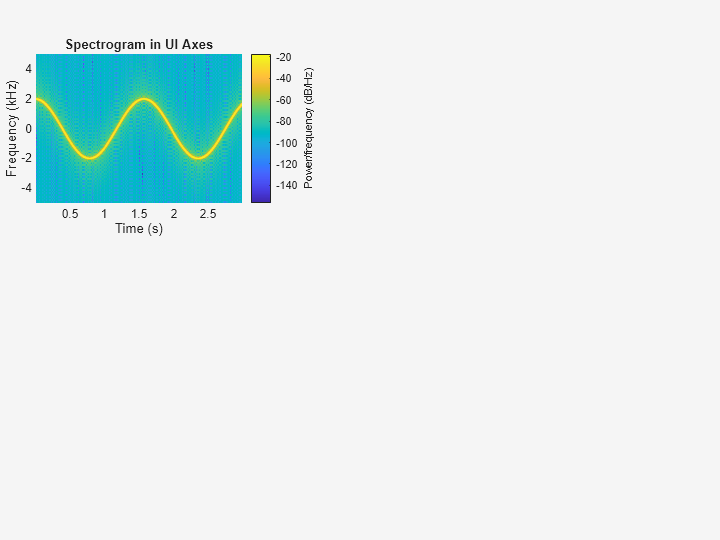
Plot Spectrogram in Target UI Axes

Create an axes in the northwestern corner of a new UI figure window.

uif = uifigure(Position=[100 100 720 540]);
ax3 = uiaxes(uif,Position=[5 305 300 200]);

Plot the PSD estimate of the signal x3 on the figure axes. Display the frequencies in the y-axis and centered at 0 kHz.

spectrogram(x3,g,ol,nfft,Fs,"centered","yaxis",Parent=ax3);
title(ax3,"Spectrogram in UI Axes")

Plot Spectrogram in Target Panel Container

Add a panel container in the southeastern corner of the UI figure window.

p = uipanel(uif,Position=[300 5 400 325], ...
    Title="Spectrogram in UI Panel", ...
    BackgroundColor="white");

Plot the PSD estimate of the signal x4 on the panel container. Display the frequencies in the y-axis.

spectrogram(x4,g,ol,nfft,Fs,"yaxis",Parent=p);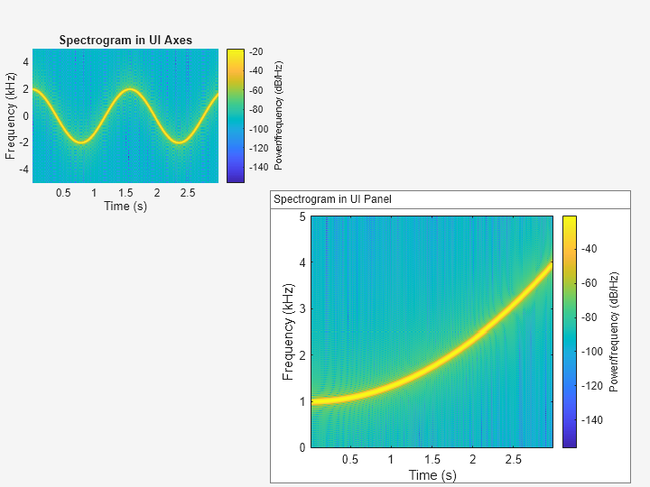

Input Arguments

x — Input signal

vector

Input signal, specified as a vector.

Example: x = chirp(0:0.001:1,0,0.5,100,"quadratic") specifies a quadratic swept-frequency signal.

Data Types: single | double
Complex Number Support: Yes

win — Window

[] (default) | positive integer | vector

Window, specified as empty ([]), a positive integer, or a vector.

The spectrogram function divides the input signal x into segments and uses a window to compute the element-by-element product of the segment samples and the window values. The window values depend on the how you specify this argument.

• Empty ([]) — spectrogram uses a Hamming window of a length such that x is divided into eight segments with nOverlap overlapping samples.

• Positive integer — spectrogram divides x into segments of length win and uses a Hamming window of that length.

• Vector — spectrogram divides x into segments of the same length as the vector win and uses the window specified in win.

If the length of x cannot be divided exactly into an integer number of segments with nOverlap overlapping samples, then spectrogram truncates x accordingly.

For a list of available windows, see Windows.

Example: hann(N+1) and (1-cos(2*pi*(0:N)'/N))/2 both specify a Hann window of length N + 1.

nOverlap — Number of overlapped samples

[] (default) | nonnegative integer

Number of overlapped samples, specified as empty ([]) or a nonnegative integer.

• Empty ([]) — spectrogram uses a number that produces 50% overlap between segments.

  If the segment length is unspecified, the function sets nOverlap to ⌊N_x / 4.5⌋, where N_x is the length of the input signal and the ⌊ ⌋ symbols denote the floor function. This action is equivalent to dividing the signal into the longest possible segments to obtain as close to but not exceed eight segments with 50% overlap.

• Nonnegative integer — spectrogram overlaps adjoining segments using the number of samples specified in this argument.

  • If win is scalar, then nOverlap must be smaller than win.

  • If win is a vector, then nOverlap must be smaller than the length of win.

freqSpec — Frequency specification

[] (default) | positive integer | vector

Frequency specification, specified as one of these values:

• Empty, [] — spectrogram calculates the spectral estimates using a number of DFT points equal to the greater of 256 or the next power of two that is equal or larger than the window length.

• Positive integer — spectrogram calculates the spectral estimates using the number of DFT points specified in this argument.

• Vector of at least two elements — spectrogram calculates the spectral estimates at the frequencies specified in freqSpec.

  • If you specify the sample rate, Fs, spectrogram assumes freqSpec as cyclical frequencies in the same units as of Fs.

  • If you do not specify Fs, spectrogram assumes freqSpec as normalized frequencies in rad/sample.

Example: freqSpec = 512 specifies 512 DFT points.

Example: freqSpec = pi./[8 4 2] specifies a vector of three normalized frequencies.

Data Types: single | double

Fs — Sample rate

positive scalar

Sample rate, specified as a positive scalar. The sample rate is the number of samples per unit time. If the unit of time is seconds, then the sample rate is in Hz.

• If you specify Fs as empty [], then spectrogram assumes that the input signal x has a sample rate of 1 Hz.

• If you do not specify Fs, then spectrogram assumes that the input signal x has a sample rate of 2π rad/sample.

freqRange — Frequency range of PSD estimate or power spectrum

"onesided" | "twosided" | "centered"

Frequency range of the PSD estimate or power spectrum, specified as "onesided", "twosided", or "centered".

The spectrogram function returns ps with a number of rows and frequency interval that depends on the value specified in freqRange, whether the number of DFT points freqSpec is even or odd, and whether Fs is specified or not.

freqRange	freqSpec	Number of Rows in ps	Frequency Interval for ps
			Fs unspecified	Fs specified
"onesided" (default if x is real-valued)	Even	freqSpec/2 + 1	[0,π] rad/sample	[0,Fs/2] cycles/unit time
	Odd	(freqSpec + 1)/2	[0,π) rad/sample	[0,Fs/2) cycles/unit time
"twosided" (default if x is complex-valued)	Even or odd	freqSpec	[0,2π) rad/sample	[0,Fs) cycles/unit time
"centered"	Even	freqSpec	(–π,π] rad/sample	(–Fs/2,Fs/2] cycles/unit time
	Odd		(–π,π) rad/sample	(–Fs/2,Fs/2) cycles/unit time

Note

• This argument is not supported if you specify freqSpec as a vector of cyclical or normalized frequencies.

• The "onesided" value is not supported if x is complex-valued.

Data Types: char | string

spectrumType — Power spectrum scaling

"psd" (default) | "power"

Power spectrum scaling, specified as one of these values:

• "psd" — spectrogram returns the power spectral density.

• "power" — spectrogram scales each estimate of the PSD by the equivalent noise bandwidth of the window and returns an estimate of the power at each frequency. If you also specify "reassigned", spectrogram integrates the PSD over the width of each frequency bin before reassigning.

This table shows the scaling relation between the PSD estimate and power spectrum estimate, either of both returned in ps, given an input signal x, window vector win, overlap length nOverlap, frequency specification freqSpec, and sample rate Fs.

Sample Rate	Scaling Relation
Fs specified	[~,~,~,psd] = spectrogram(x,win,nOverlap,freqSpec,Fs,"psd"); [~,~,~,pow] = spectrogram(x,win,nOverlap,freqSpec,Fs,"power"); Then, pow is equivalent to psd*enbw(win,Fs).
Fs unspecified	[~,~,~,psd] = spectrogram(x,win,nOverlap,freqSpec,"psd"); [~,~,~,pow] = spectrogram(x,win,nOverlap,freqSpec,"power"); Then, pow is equivalent to psd*enbw(win,2*pi).

Data Types: char | string

Name-Value Arguments

Specify optional pairs of arguments as Name1=Value1,...,NameN=ValueN, where Name is the argument name and Value is the corresponding value. Name-value arguments must appear after other arguments, but the order of the pairs does not matter.

Example: spectrogram(x,100,OutputTimeDimension="downrows") divides x into segments of length 100 and windows each segment with a Hamming window of that length The output of the spectrogram has time dimension down the rows.

MinThreshold — Threshold

-Inf (default) | real scalar

Threshold, specified as a real scalar expressed in decibels.

If you specify MinThreshold=th, spectrogram sets to zero those elements of s that satisfy the condition 10 log₁₀(s) ≤ th.

OutputTimeDimension — Output time dimension

"acrosscolumns" (default) | "downrows"

Output time dimension, specified as one of these values:

• "acrosscolumns" — spectrogram sets the time dimension of s, ps, fc, and tc across the columns and the frequency dimension along the rows.

• "downrows" — spectrogram sets the time dimension of s, ps, fc, and tc down the rows and the frequency dimension along the columns.

This argument is ignored if you use spectrogram with output arguments.

Data Types: char | string

Parent — Target parent container

[] (default) | Axes object | UIAxes object | Panel object

Since R2025a

Target parent container, specified as an Axes object, a UIAxes object, or a Panel object.

If you specify Parent, the spectrogram function draws the spectrogram in the specified target parent container, whether you call the function with or without output arguments.

For more information about target containers and the parent-child relationship in MATLAB^® graphics, see Graphics Object Hierarchy. For more information about using Parent in UIAxes and Panel objects to design apps, see Plot Spectral Representations of Signal in App Designer.

Output Arguments

s — STFT output

matrix

Short-time Fourier transform (STFT) output, returned as a matrix. Time increases across the columns of s and frequency increases down the rows, starting from zero.

• If x is a signal of length N_x, then s has k columns, where

  • k = ⌊(N_x – nOverlap)/(win – nOverlap)⌋ if win is a scalar.

  • k = ⌊(N_x – nOverlap)/(length(win) – nOverlap)⌋ if win is a vector.

• If x is real-valued and freqSpec is even, then s has (freqSpec/2 + 1) rows.

• If x is real-valued and freqSpec is odd, then s has (freqSpec + 1)/2 rows.

• If x is complex-valued, then s has freqSpec rows.

• s remains unchanged if you specify the "reassigned" argument.

Note

If you set freqRange to "onesided", spectrogram outputs the s values in the positive Nyquist range and does not conserve the total power.

f — Frequencies associated with STFT output

vector

Frequencies associated with the STFT output, returned as a vector.

• If you specify Fs, then f contains cyclical frequencies in Hz.

• If you do not specify Fs, then f contains normalized frequencies in rad/sample.

t — Times associated with STFT output

vector

Times associated with the STFT output, returned as a vector.

• If you specify Fs, then t contains time instants in seconds.

• If you do not specify Fs, then t contains sample indices in (sample numbers)/(2π).

The values in t correspond to the midpoint of each segment.

ps — Power spectral density or power spectrum

matrix

Power spectral density (PSD) or power spectrum, returned as a matrix.

• If x is real-valued and you do not specify freqRange or set it to "onesided", then ps contains the one-sided modified periodogram estimate of the PSD or power spectrum of each segment. The function multiplies the power by 2 at all frequencies except 0 and the Nyquist frequency to conserve the total power.

• If x is complex-valued or if you set freqRange to "twosided" or "centered", then ps contains the two-sided modified periodogram estimate of the PSD or power spectrum of each segment.

• If you specify a vector of normalized frequencies or cyclical frequencies in freqSpec, then ps contains the modified periodogram estimate of the PSD or power spectrum of each segment evaluated at the input frequencies.

fc, tc — Center-of-energy frequencies and times

matrices

Center-of-energy frequencies and times, returned as matrices of the same size as the short-time Fourier transform. If you do not specify a sample rate, then the elements of fc are returned as normalized frequencies.

The spectrogram function returns fc and tc only if you specify the "reassigned" option. If each reassigned value in fc or tc is out of range, spectrogram replaces them with the corresponding values from f and t, respectively.

More About

Short-Time Fourier Transform

The short-time Fourier transform (STFT) is used to analyze how the frequency content of a nonstationary signal changes over time. The magnitude squared of the STFT is known as the spectrogram time-frequency representation of the signal. For more information about the spectrogram and how to compute it using Signal Processing Toolbox™ functions, see Spectrogram Computation with Signal Processing Toolbox.

The STFT of a signal is computed by sliding an analysis window g(n) of length M over the signal and calculating the discrete Fourier transform (DFT) of each segment of windowed data. The window hops over the original signal at intervals of R samples, equivalent to L = M – R samples of overlap between adjoining segments. Most window functions taper off at the edges to avoid spectral ringing. The DFT of each windowed segment is added to a complex-valued matrix that contains the magnitude and phase for each point in time and frequency. The STFT matrix has

$$k=\lfloor \frac{N_x-L}{M-L}\rfloor$$

columns, where N_x is the length of the signal x(n) and the ⌊⌋ symbols denote the floor function. The number of rows in the matrix equals N_DFT, the number of DFT points, for centered and two-sided transforms and an odd number close to N_DFT/2 for one-sided transforms of real-valued signals.

The mth column of the STFT matrix $$X(f)=\left[\begin{array}{ccccc}{X}_1(f)& X_2(f)& X_3(f)& \cdots & X_k(f)\end{array}\right]$$ contains the DFT of the windowed data centered about time mR:

$$X_m(f)={\displaystyle \sum _{n=-\infty }^{\infty }x(n)g(n-mR)e^{-j2\pi fn}}.$$

Tips

• If an STFT matrix has zeros, its conversion to decibels results in negative infinities that cannot be plotted. To avoid this issue, spectrogram adds eps to the STFT matrix when you call it with no output arguments or by specifying the Parent argument.

• If an STFT matrix has magnitude values very close to zero and you specify the "reassigned" option, the spectrogram reassignment can be numerically sensitive. In such cases, do not use the "reassigned" option.

References

[1] Boashash, Boualem, ed. Time Frequency Signal Analysis and Processing: A Comprehensive Reference. Second edition. EURASIP and Academic Press Series in Signal and Image Processing. Amsterdam and Boston: Academic Press, 2016.

[2] Chassande-Motin, Éric, François Auger, and Patrick Flandrin. "Reassignment." In Time-Frequency Analysis: Concepts and Methods. Edited by Franz Hlawatsch and François Auger. London: ISTE/John Wiley and Sons, 2008.

[3] Fulop, Sean A., and Kelly Fitz. "Algorithms for computing the time-corrected instantaneous frequency (reassigned) spectrogram, with applications." Journal of the Acoustical Society of America. Vol. 119, January 2006, pp. 360–371.

[4] Oppenheim, Alan V., and Ronald W. Schafer, with John R. Buck. Discrete-Time Signal Processing. Second edition. Upper Saddle River, NJ: Prentice Hall, 1999.

[5] Rabiner, Lawrence R., and Ronald W. Schafer. Digital Processing of Speech Signals. Englewood Cliffs, NJ: Prentice-Hall, 1978.

Extended Capabilities

Tall Arrays

Calculate with arrays that have more rows than fit in memory.

The spectrogram function supports tall arrays with the following usage notes and limitations:

• Input must be a tall column vector.

• The win argument must always be specified.

• OutputTimeDimension must be always specified and set to "downrows".

• The reassigned option is not supported.

• The fc and tc output arguments are not supported.

• The Parent argument is not supported.

• Syntaxes with no output arguments are not supported.

For more information, see Tall Arrays.

C/C++ Code Generation

Generate C and C++ code using MATLAB® Coder™.

Usage notes and limitations:

• The Parent input argument is not supported.

• Arguments specified using name-value arguments must be compile-time constants.

GPU Code Generation

Generate CUDA® code for NVIDIA® GPUs using GPU Coder™.

Usage notes and limitations:

• Arguments specified using name-value arguments must be compile-time constants.

• Variable-size win must be double precision.

Thread-Based Environment

Run code in the background using MATLAB® backgroundPool or accelerate code with Parallel Computing Toolbox™ ThreadPool.

The spectrogram function supports thread-based environments with these usage notes and limitations:

• The syntax with no output arguments is not supported.

• The frequency vector must be uniformly spaced.

For more information, see Run MATLAB Functions in Thread-Based Environment.

GPU Arrays

Accelerate code by running on a graphics processing unit (GPU) using Parallel Computing Toolbox™.

This function fully supports GPU arrays. For more information, see Run MATLAB Functions on a GPU (Parallel Computing Toolbox).

Version History

Introduced before R2006a

R2025a: Visualize function outputs in specified parent targets

The spectrogram function supports plotting output in a parent axes or panel container specified using the Parent input argument.

R2024a: Code generation support for single-precision variable-size window inputs

The spectrogram function supports single-precision variable-size window inputs for code generation.

R2023b: spectrogram supports single-precision data and GPU code generation

The spectrogram function supports single-precision inputs and code generation for graphical processing units (GPUs). You must have MATLAB Coder™ and GPU Coder™ to generate CUDA^® code.

R2023a: Visualize function outputs using Create Plot Live Editor task

You can now use the Create Plot Live Editor task to visualize the output of spectrogram interactively. You can select different chart types and set optional parameters. The task also automatically generates code that becomes part of your live script.