binscatter

R2026b

Binned scatter plot

• 

Syntax

binscatter(x,y)

binscatter(x,y,N)

binscatter(tbl,xvar,yvar)

binscatter(tbl,xvar,yvar,N)

binscatter(___,Name=Value)

binscatter(ax,___)

h = binscatter(___)

Description

Vector Data

binscatter(x,y) displays a binned scatter plot of x and y. A binned scatter plot partitions the data space into rectangular bins and displays each bin as a tile. The bin counts are indicated by the color or opacity of the tile, depending on the number of data sets you plot. If you zoom into the plot, the tile sizes automatically adjust to show finer resolution.

• To plot one data set, specify x and y as vectors of the same length. Within the resulting distribution, the tile colors come from a colormap, with color indicating the bin counts.

• To plot multiple data sets, specify at least one of x or y as a matrix. Each resulting distribution displays a different color. Within a distribution, variations in opacity indicate the bin counts. (since R2026b)

binscatter(x,y,N) specifies the number of bins to use. N can be a scalar or a two-element vector [Nx Ny]. If N is a scalar, then Nx and Ny are both set to the scalar value. The maximum number of bins in each dimension is 250.

Table Data

Since R2026a

binscatter(tbl,xvar,yvar) creates a binned scatter plot using the variables xvar and yvar from the table tbl. To plot multiple data sets, specify multiple table variable indices for xvar, yvar, or both.

binscatter(tbl,xvar,yvar,N) plots the table data using the specified number of bins.

Additional Options

binscatter(___,Name=Value) specifies property values with one or more name-value pair arguments. For example, binscatter(x,y,ShowEmptyBins="on") colors areas with no data points. For a full list of properties, see Binscatter Properties. Use this option with any of the input argument combinations in previous syntaxes.

binscatter(ax,___) plots into the axes specified by ax instead of into the current axes (gca). The ax input can precede any of the input argument combinations in previous syntaxes.

h = binscatter(___) returns a Binscatter object. Use this object to inspect and adjust the properties of the binned scatter plot.

Examples

Binned Scatter Plot of Vectors

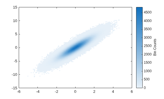
Generate random numbers in both the x and y dimensions and create a binned scatter plot. The binscatter function automatically chooses an appropriate number of bins to cover the range of values in the data.

x = randn(1e6,1);
y = 2*x + randn(1e6,1);
binscatter(x,y)

Specify Number of Bins

Plot a binned scatter plot of 10,000 random numbers sorted into 30 bins in the x dimension and 10 bins in the y dimension.

rng default % for reproducibility
x = randn(1e4,1);
y = randn(1e4,1);
h = binscatter(x,y,[30 10]);

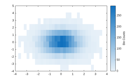
Find the bin counts. The result is a matrix with the top left element corresponding to the bin count of the bottom left bin in the plot. The x bins are in the rows of the matrix and the y bins are in the columns.

counts = h.Values;

Binned Scatter Plot from Table

Since R2026a

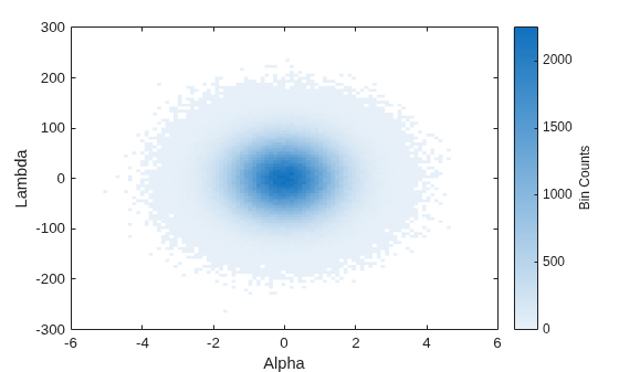
Create a table and plot the variables. When you pass a table to the binscatter function, the axis labels display the variable names.

Alpha = randn(1e6,1);
Lambda = 50*randn(1e6,1);
tbl = table(Alpha,Lambda);
binscatter(tbl,"Alpha","Lambda")

Change Color Map of Binned Scatter Plot

Create a binned scatter plot of some random data points.

x = randn(1e5,1);
y = randn(1e5,1);
binscatter(x,y)

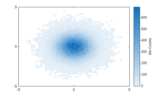
The default color map ranges from light colors (for small values) to dark colors (for large values). Switching to a color map that uses dark colors for small values can make it easier to spot outliers.

Use the colormap function to change the colors in the plot. Pass in the current axes handle using gca.

colormap(gca,"parula")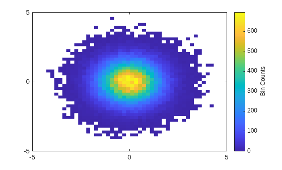

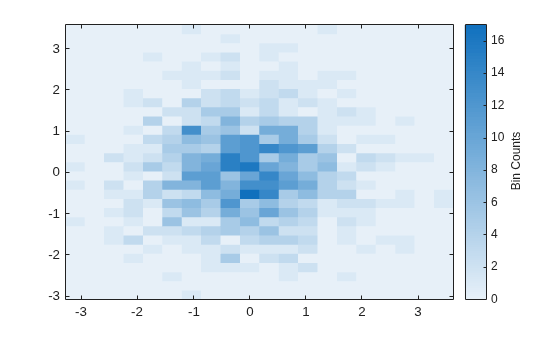
Adjust Binned Scatter Plot Properties

Generate 1,000 random numbers and create a binned scatter plot. Return the Binscatter object to adjust properties of the plot without recreating the entire plot.

x = randn(1000,1);
y = randn(1000,1);
h = binscatter(x,y)

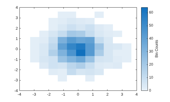
h = 
  Binscatter with properties:

      NumBins: [11 11]
    XBinEdges: [-3.2764 -2.6485 -2.0206 -1.3927 -0.7648 -0.1369 0.4910 1.1189 1.7468 2.3747 3.0026 3.6305]
    YBinEdges: [-3.1155 -2.5034 -1.8914 -1.2794 -0.6674 -0.0553 0.5567 1.1687 1.7808 2.3928 3.0048 3.6168]
       Values: [11×11 double]
      XLimits: [-3.2764 3.6305]
      YLimits: [-3.1155 3.6168]
    FaceAlpha: 1

  Show all properties

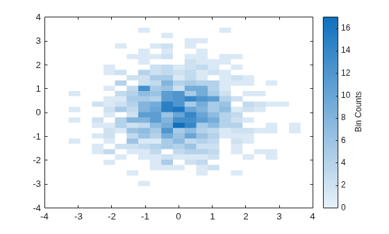
Specify exactly how many bins to use in each direction.

h.NumBins = [20 30];

Turn on the display of empty bins in the plot.

h.ShowEmptyBins = "on";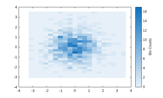

Specify the extent of the axes with the XLimits and YLimits properties. Then limit the bin limits in the x direction with a vector.

xlim(gca,h.XLimits);
ylim(gca,h.YLimits);
h.XLimits = [-1 1];

Multiple Binned Scatter Plots

Since R2026b

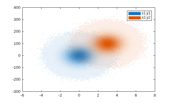
One way to plot multiple binned scatter plots is to specify x and y as matrices of the same size, where each pair of corresponding columns represents a different data set. Another way is to use the hold on command between calls to binscatter, but this approach requires specifying some name-value arguments. This example shows both techniques.

Create two vectors of x-values and two vectors of y-values. Then use them to create two matrices of data to plot.

x1 = randn(1e6,1);
x2 = randn(1e6,1) + 3;
y1 = 50*randn(1e6,1);
y2 = 50*randn(1e6,1) + 100;
x = [x1 x2];
y = [y1 y2];

Plot both matrices and add a legend. Each distribution has a different overall hue, and within each distribution, the tiles vary in opacity according to the bin counts. Higher bin counts have a more opaque, intense color.

figure
binscatter(x,y)
legend("x1,y1","x2,y2")

Now plot two distributions using the hold on command after the first call to binscatter.

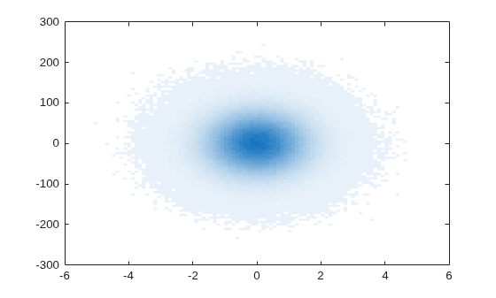
Plot the x1 and y1 vectors. Ensure that the plot displays the same hue with different tile opacities by specifying the FaceAlpha name-value argument as "flat".

figure
b1 = binscatter(x1,y1,FaceAlpha="flat");
hold on

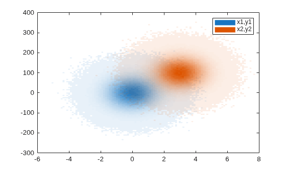
Plot the second data set. Then add a legend.

binscatter(x2,y2,FaceAlpha="flat")
legend("x1,y1","x2,y2")
hold off

Input Arguments

x, y — Input data

vectors | matrices | vector and matrix

Input data, specified vectors of the same length, matrices of the same size, or a vector and a matrix that share the same length in one dimension. The values of x and y must be real.

This table shows how the different shapes of x and y affect the default (light theme) appearance of a plot. You can change the plot colors and opacity by setting the FaceColor and FaceAlpha properties.

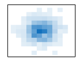
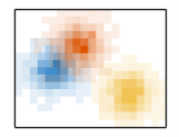
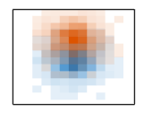
x and y	Result	Appearance
Two vectors of the same length	One binned scatter plot that uses a colormap to distinguish bin counts. The default colormap is sky (in the light theme) or abyss (in the dark theme). By default, a colorbar showing the correspondence between the colors and the bin counts appears next to the plot (not shown in the illustration).
Two matrices of the same size	Multiple binned scatter plots, each with a different color. Within each plot, the tile opacity varies from translucent (low count) to fully opaque (high count). By default, the colors repeat after seven plots. You can specify other color palettes that have more colors by using the colororder function. Use the legend function to distinguish each data set instead of a colorbar.
A vector and a matrix that share the same length in one dimension	Multiple binned scatter plots that share one set of coordinates. Each plot has a different color. Within each plot, the tile opacity varies from translucent (low count) to fully opaque (high count). By default, the colors repeat after seven plots. You can specify other color palettes that have more colors by using the colororder function. Use the legend function to distinguish each data set.

Data Types: single | double | int8 | int16 | int32 | int64 | uint8 | uint16 | uint32 | uint64 | logical | datetime | duration

tbl — Source table

table | timetable

Source table containing the data to plot, specified as a table or timetable.

xvar, yvar — Table variables containing x- and y-coordinates

one or more table variable indices each

Table variables containing the x- and y-coordinates, specified as one or more table variable indices each. The table variables you specify can contain numeric, logical, datetime, or duration values. Within each argument, the specified variables must have the same type. If you specify multiple table variable indices for both xvar and yvar, the number of indices must match.

Specify the table variable indices using any of the following indexing schemes.

Indexing Scheme	Examples
Variable names: A string array, character vector, or cell array. A pattern object.	"A" or 'A' — A variable named A ["A","B"] or {'A','B'} — Two variables named A and B "Var"+digitsPattern(1) — Variables named "Var" followed by a single digit
Variable indices: An index number that refers to the location of a variable in the table. A vector of numbers. A logical vector. Typically, this vector is the same length as the number of variables, but you can omit trailing 0 or false values.	3 — The third variable from the table [2 3] — The second and third variables from the table [false false true] — The third variable
Variable type: A vartype subscript that selects variables of a specified type.	vartype("double") — All the variables containing double values

Plot One or Multiple Data Sets

Binned scatter plots have a different appearance depending on whether you specify one table variable index each or multiple table variables.

This table shows the default (light theme) appearance of plots created from one or multiple table variables. You can change the plot colors and opacity by setting the FaceColor and FaceAlpha properties.

xvar and yvar	Result	Appearance
One table variable index each	One binned scatter plot that uses a colormap to distinguish bin counts. The default colormap is sky (in the light theme) or abyss (in the dark theme). By default, a colorbar showing the correspondence between the colors and the bin counts appears next to the plot (not shown in the illustration).
Multiple table variable indices each (since R2026b)	Multiple binned scatter plots, each with a different color. Within each plot, the tile opacity varies from translucent (low count) to fully opaque (high count). By default, the colors repeat after seven plots. You can specify other color palettes that have more colors by using the colororder function. Use the legend function to distinguish each data set instead of a colorbar.
One table variable index for either xvar or yvar, and multiple indices for the other argument (since R2026b)	Multiple binned scatter plots that share one set of coordinates. Each plot has a different color. Within each plot, the tile opacity varies from translucent (low count) to fully opaque (high count). By default, the colors repeat after seven plots. You can specify other color palettes that have more colors by using the colororder function. Use the legend function to distinguish each data set.

Example: binscatter(tbl,"Input","Output") specifies the table variable named "Input" for the x-coordinates and the variable named "Output" for the y-coordinates.

Example: binscatter(tbl,2,"Output") specifies the second table variable for the x-coordinates and the variable named "Output" for the y-coordinates.

Example: binscatter(tbl,["X1","X2"],["Y1","Y2"]) specifies two table variables for the x-coordinates and two table variables for the y-coordinates. (since R2026b)

N — Number of bins

scalar | two-element vector

Number of bins, specified as a scalar or two-element vector [Nx Ny].

• If N is a two-element vector [Nx Ny], then binscatter uses Nx bins in the x dimension and Ny bins in the y dimension.

• If N is a scalar, then Nx and Ny are both set to the scalar value.

binscatter uses Nx and Ny bins along the x and y dimensions in the initial plot, when the axes are not zoomed in. (The axes are not zoomed in when the XLimMode and YLimMode properties are both "auto".) When zooming, binscatter adjusts the number of bins to maintain a bin size such that the visible portion of the plot is approximately divided into Nx-by-Ny bins.

The maximum number of bins in each dimension is 250. The default number of bins is computed based on the data size and standard deviation and does not exceed 100.

Example: [10 20]

Data Types: single | double | int8 | int16 | int32 | int64 | uint8 | uint16 | uint32 | uint64

ax — Target axes

gca (default) | Axes object

Target axes, specified as an Axes object. If you do not specify the axes, then binscatter uses the current axes (gca).

Name-Value Arguments

Specify optional pairs of arguments as Name1=Value1,...,NameN=ValueN, where Name is the argument name and Value is the corresponding value. Name-value arguments must appear after other arguments, but the order of the pairs does not matter.

Example: binscatter(x,y,ShowEmptyBins="on") turns on the display of empty bins in the plot.

The properties listed here are only a subset. For a complete list, see Binscatter Properties.

XLimits — Data limits in x-dimension

vector

Data limits in x-dimension, specified as a two-element vector [Xmin Xmax].

binscatter only displays data points that fall within the specified data limits inclusively, $$X_{\min }\le X\le X_{\max }$$.

Example: [0 10]

Data Types: single | double | int8 | int16 | int32 | int64 | uint8 | uint16 | uint32 | uint64 | datetime | duration

YLimits — Data limits in y-dimension

vector

Data limits in y-dimension, specified as a two-element vector [Ymin Ymax].

binscatter only displays data points that fall within the specified data limits inclusively, $$Y_{\min }\le Y\le Y_{\max }$$.

Example: [0 10]

Data Types: single | double | int8 | int16 | int32 | int64 | uint8 | uint16 | uint32 | uint64 | datetime | duration

ShowEmptyBins — Toggle to show empty bins

"off" (default) | on/off logical value

Toggle to show empty bins, specified as either "off" or "on", or as numeric or logical 1 (true) or 0 (false). A value of "on" is equivalent to true, and "off" is equivalent to false. Thus, you can use the value of this property as a logical value. The value is stored as an on/off logical value of type matlab.lang.OnOffSwitchState.

Specify "on" or true to color tiles in the plot that fall within the bin limits, but have no data points.

FaceColor — Tile color

"flat" | color name or short name | RGB triplet | hexadecimal color code | "none"

Since R2026b

Tile color, specified as one of these values:

• "flat" — Tile colors vary according to the bin counts. By default, the colors come from the sky colormap (in the light theme) or the abyss colormap (in the dark theme). You can change the colormap by calling the colormap function after plotting.

• Color name (or short name) — Tiles have a uniform color. Specify "red" (or "r"), "green" (or "g"), "blue" (or "b"), "cyan" (or "c"), "magenta" (or "m"), "yellow" (or "y"), "black" (or "k"), or "white" (or "w").

• RGB triplet — Tiles have a uniform color. An RGB triplet is a three-element row vector whose elements specify the intensities of the red, green, and blue components of the color. The intensities must be in the range [0,1]; For example, [0.4 0.6 0.7].

• Hexadecimal color code — Tiles have a uniform color. A hexadecimal color code is a string scalar or character vector that starts with a hash symbol (#) followed by three or six hexadecimal digits, which can range from 0 to F. The values are not case sensitive. The color codes "#FF8800", "#ff8800", "#F80", and "#f80" are equivalent.

• "none" — Tiles have no color.

This table lists the default color palettes for plots in the light and dark themes. You can use the colors from these palettes to match other plots.

Palette	Palette Colors
"gem" — Light theme default Before R2025a: Most plots use these colors by default.
"glow" — Dark theme default

To get the RGB triplets and hexadecimal color codes for these palettes , use the orderedcolors and rgb2hex functions. For example, get the RGB triplets for the "gem" palette and convert them to hexadecimal color codes.

RGB = orderedcolors("gem");
H = rgb2hex(RGB);

Example: binscatter(x,y,FaceColor="g") creates a binned scatter plot with green tiles.

Example: binscatter(x,y,FaceColor="#8B6CE0") creates a binned scatter plot with purple tiles.

Example: binscatter(x,y,FaceColor="flat") creates a binned scatter plot with tile colors that vary according to the bin counts.

FaceAlpha — Transparency of tiles

"flat" (since R2026b) | scalar in the range [0, 1]

Transparency of the tiles, specified as "flat" or as a scalar in the range [0, 1].

• "flat" — Vary the tile transparency according to the bin counts, where more opaque bins have higher counts. You can adjust the mapping of bin counts to the transparency levels using the alpha and alphamap functions. Specifying the FaceAlpha value as "flat" can cause the FaceColor property to change to a uniform color for all the bins instead of using a colormap. This change happens when the FaceColorMode property of the Binscatter object has a value of "auto" (the default value).

• Scalar in the range [0, 1] — Use the same transparency for all the tiles. A value of 1 means fully opaque and 0 means completely transparent (invisible).

Example: binscatter(x,y,FaceAlpha=0.5) creates a binned scatter plot with semitransparent bins.

Example: binscatter(x,y,FaceAlpha="flat") creates a binned scatter plot with tile transparencies that vary according to the bin counts. (since R2026b)

Output Arguments

h — Binscatter object

Binscatter object

Binscatter object. Use this object to inspect and adjust properties of the plot. For a full listing of properties, see Binscatter Properties.

Tips

• Change the ColorScale property of the axes to "log" to produce better bin coloring when a few bins dominate the plot.

  ax = gca;
  ax.ColorScale = "log";

Extended Capabilities

Tall Arrays

Calculate with arrays that have more rows than fit in memory.

The binscatter function supports tall arrays with the following usage notes and limitations:

• Tall tables and tall timetables are not supported.

• If you specify your data as a tall array, the binscatter function plots in iterations, progressively adding to the plot as more data is read. During the updates, a progress indicator shows the proportion of data that has been plotted. Zooming and panning is supported during the updating process, before the plot is complete. To stop the update process, press the pause button in the progress indicator.

For more information, see Tall Arrays.

Version History

Introduced in R2017b

R2026b: Create multiple plots

Create binned scatter plots from multiple data sets simultaneously by specifying the input data as two matrices, a vector and a matrix, or multiple table variables. Each plot has a different overall hue, and the tiles of each plot vary in opacity according to the bin counts. For an example, see Multiple Binned Scatter Plots.

R2026a: Pass tables directly to binscatter

Create plots by passing a table to the binscatter function followed by the variables you want to plot. When you specify the data as a table, the axis labels display the table variable names automatically.

R2025a: Plots in UI axes use sky colormap

When you create a binned scatter plot using a UIAxes object, the plot colors come from the sky colormap. Previously, the plot colors came from the parula colormap.