Explore 3-D Volumetric Data with Volume Viewer

This example shows how to look at and explore 3-D volumetric data using the Volume Viewer app. Volume rendering is highly dependent on defining an appropriate alphamap so that structures in your data that you want to see are opaque and structures that you do not want to see are transparent. To illustrate, the example loads an MRI study of the human head into the Volume Viewer app and explores the data using the visualization capabilities of the Volume Viewer.

• Load Volume Data into the Volume Viewer

• View Volume Data in Volume Viewer

• Adjust View of Volume Data in Volume Viewer

• Refine View with Rendering Editor

• Save Volume Viewer Rendering and Camera Configuration Settings

• Apply Rendering and Camera Configuration Settings Outside the App

Load Volume Data into Volume Viewer

This part of the example shows how to load volumetric data into the Volume Viewer app.

Load the MRI data of a human head from a MAT file into the workspace. The MRI data is a modified subset of the BraTS data set [1]. This operation creates a variable named D in your workspace that contains the volumetric data. Use the squeeze command to remove the singleton dimension from the data.

load mri
D = squeeze(D);
whos

  Name        Size                 Bytes  Class     Attributes

  D         128x128x27            442368  uint8               
  map        89x3                   2136  double              
  siz         1x3                     24  double              

Open the Volume Viewer app. From the MATLAB® Toolstrip, open the Apps tab and, under Image Processing and Computer Vision, click . You can also open the app by using the volumeViewer command.

volumeViewer

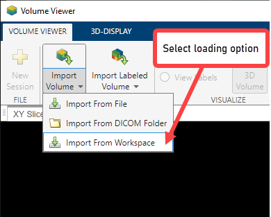
Load volumetric data into the Volume Viewer app. You can load an image by specifying its filename or by loading a variable from the workspace. Loading from a file is useful when the file contains metadata specifying the voxel spacing, especially if the voxel spacing is anisotropic (nonuniform between dimensions). If you have volumetric data in a DICOM format that uses multiple files to represent a volume, you can specify the DICOM folder name. In the Viewer tab of the app toolstrip, click Import. For this example, under Data, choose From Workspace because the data is already in the workspace.

Select the workspace variable D in the Import Volume dialog box and click OK.

View Volume Data in Volume Viewer

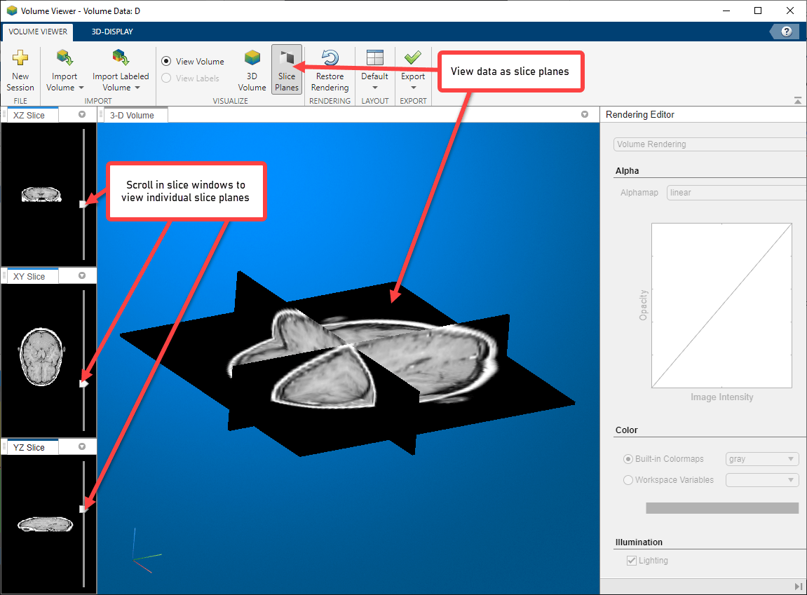
By default, Volume Viewer displays the data as three 2-D slice planes and a 3-D volume in a four-pane view. You can change the layout to focus on one pane by selecting Layout in the app toolstrip and, under Focus, the pane you want to focus on.

To explore the volume, zoom in and out on any of the display panes using the mouse wheel, or by selecting the zoom icon in the top-right corner of the pane and clicking the image. Navigate between 2-D slices by using the scroll bar in each of the 2-D slice panes. Labels in the bottom-left corner of each slice pane indicate the current slice number and the total number of slices in that dimension. The bottom of the app window displays information about the pixel beneath the mouse pointer, including its coordinates and intensity.

In the 3-D Volume pane, you can drag the volume to rotate it about its center. The orientation axes in the bottom-left corner indicate the spatial orientation of the volume. The scale bar in the bottom-right corner provides an indication of the volume size. You can toggle the visibility of the orientation axes and scale bar by selecting Display Markers in the app toolstrip and selecting or clearing options.

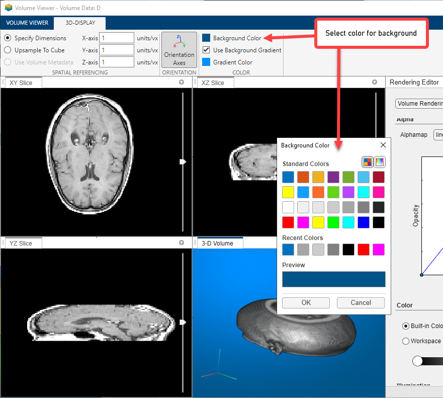
You can change the background color or apply a background gradient to the 3-D Volume pane from the 3-D Display tab of the app toolstrip. To change the background color, select the down-arrow next to Background Color and select a color. Clear or select Use Background Gradient to toggle whether the pane applies a gradient to the background using a second color. To change the gradient color, select the down-arrow next to Gradient Color and select a color.

Adjust Voxel Spacing of Volume Data in Volume Viewer

By default, the app assumes uniform voxel spacing of 1-by-1-by-1 mm. If you know your volume has different spacing, you can specify it to display the volume using the correct scaling.

You can specify custom voxel spacing in the 3-D Display tab using one of these options:

• Specify Dimensions — Specify the voxel spacing in the X-, Y-, and Z-directions by entering the spacing values, in world units per voxel, in the X-axis, Y-axis, and Z-axis parameters in the toolstrip, respectively.

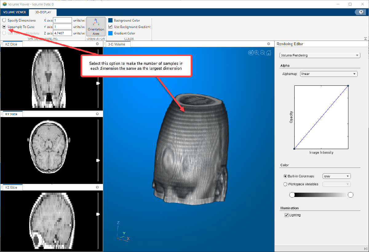
• Upsample To Cube — Display the volume using a scale factor that makes the number of slices in each dimension the same as the largest dimension in the volume. This option assumes that the field of view of the volume in world coordinates is a cube. For some volumes, this setting can make anisotropically sampled data appear more correctly scaled.

• Use Volume Metadata — Apply metadata from an imported image file to automatically scale the volume. This option is available only when you import a volume from a file, and this is the default behavior if metadata is present in the file.

Refine View with Rendering Editor

This part of the example describes how to use the Rendering Editor to modify your view of the data. Using the Rendering Editor, you can:

• Choose the rendering technique from these options: Gradient Opacity (default), Volume Rendering, Cinematic Rendering, Minimum Intensity Projection, Maximum Intensity Projection, Isosurface, and Slice Planes.

• Modify the transparency alphamap by specifying a preset alphamap, such as CT_Bone, or by customizing the alphamap using the intensity-opacity curve.

• Modify the colormap by specifying a built-in colormap like jet or CT_Bone, or by importing a colormap from the workspace. You can refine the colormap using the interactive color bar scale.

Choose the Rendering Technique

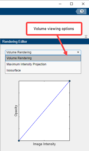
Volume Viewer offers several rendering techniques for volumes.

• Volume Rendering — View the volume based on the color and transparency for each voxel specified by the colormap and alphamap.

• Cinematic Rendering — View the volume based on the specified color and transparency for each voxel, with iterative postprocessing that produces photorealistic shadows and lighting. This technique is useful for displaying opaque volumes, but can take longer to render.

• Minimum Intensity Projection — View the voxel with the smallest intensity value for each ray projected through the data.

• Maximum Intensity Projection — View the voxel with the largest intensity value for each ray projected though the data. This technique can be useful for revealing the highest-intensity structure within a volume.

• Gradient Opacity (default) — View the volume based on the specified color and transparency, with an additional transparency applied if the voxel is similar in intensity to the previous voxel along the ray projected through the data. When you render a volume with uniform intensity using this technique, the interior appears more transparent than when displayed using Volume Rendering, enabling better visualization of intensity gradients within the volume.

• Isosurface — View the volume as an isosurface. The default isovalue is 0.5.

• Slice Planes — View the volume as three orthogonal slice planes. You can change the position of each slice by pausing on a slice plane until it highlights, and then dragging it.

Specify the Alphamap

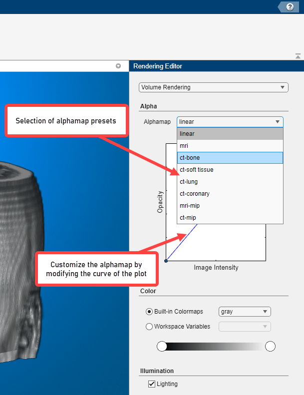
Volume rendering is highly dependent on defining an appropriate alphamap so that structures you want to see are opaque and structures you do not want to see are transparent. The Rendering Editor enables you to define the opacity and transparency of voxel values throughout the volume. As a starting point, you can choose from a set of alphamap presets that automatically achieve certain well-defined effects. For example, to define a view that generally works well with CT bone data, select the CT_Bone rendering preset. By default, Volume Viewer uses a simple linear relationship, but each preset changes the curve of the plot to give certain data values more or less opacity. You can then customize the alphamap to work well for your volume by manipulating the plot directly. The amount of adjustment required depends on the intensity range and distribution of your data.

The plot maps voxel intensity to opacity for points defined by circular sliders. For example, the default linear alphamap has two circular sliders and maps the intensity value 0 to an opacity of 0 and an intensity of 1 to an opacity of 1. The app interpolates opacity values for intensities between the circular sliders. You can add sliders by clicking the line plot. You can change the intensity associated with a slider you have created by dragging it left or right on the plot, or by selecting it and entering a new value for Intensity. You can change the opacity associated with a slider by dragging it up and down on the plot, or by selecting it and entering a new value for Opacity. Red vertical lines indicate the minimum and maximum intensities within your volume, which you can use as a guide when customizing the plot for your data.

Specify the Colormap

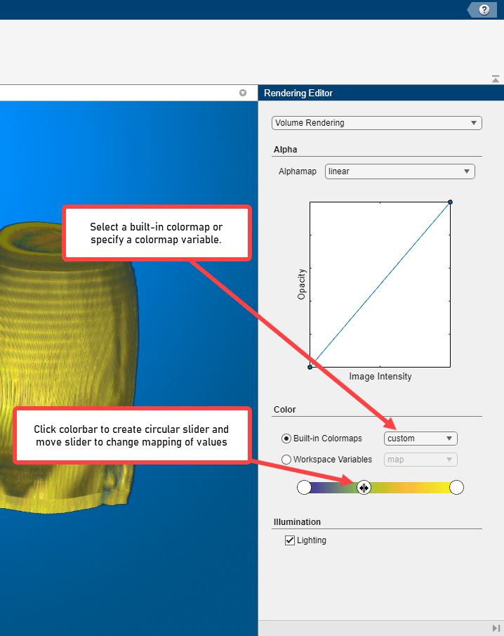
Color, when used with voxel intensity and opacity, is an important element of volume visualization. In the Rendering Editor, you can select from a list of predefined MATLAB colormaps, such as jet and parula, as well as presets that work well with medical data, such as CT_Bone. You can also specify a custom colormap that you have defined as a variable in the workspace. You can refine the color mapping for any colormap by using the interactive color bar scale. For example, to lighten the color values in a visualization, click the color bar to create a circular slider, and then drag the slider to the left. You can create multiple sliders on the color bar to further define the color mapping. The color under the line of the intensity-opacity plot updates to reflect the updated colormap.

Save Volume Viewer Rendering and Camera Configuration Settings

After configuring Volume Viewer for the best view of your data, you can save your rendering settings and camera configuration to the workspace. You can apply the saved settings to recreate the view you achieved in Volume Viewer by using them to set properties of the objects created by the viewer3d and volshow functions.

To save rendering and camera configuration settings, in the Viewer tab of the app toolstrip, click Export Settings.

Volume Viewer creates separate structures for the settings of objects created by viewer3d and volshow. In the Export To Workspace dialog box, you can choose which structures to create, and either specify their names or accept the default names of sceneConfig and objectConfig, respectively. When you are ready to export, click OK.

Apply Rendering and Camera Configuration Settings Outside App

Programmatically display the volume, applying the rendering and camera settings outside the app. The new display has the same colormap, alphamap, rendering style, background color and gradient, and camera position as the 3-D Volume pane had when you exported the settings. Note that this example loads and applies rendering settings attached to the example as a supporting file.

load("intensityVolSettings.mat")

% Create volume display

viewer = viewer3d;

Volume = volshow(D,Parent=viewer, ...
    DisplayRangeMode="data-range");

% Apply objectConfig settings by setting Volume object properties

fields = fieldnames(objectConfig);

for i = 1:numel(fields)
    Volume.(fields{i}) = objectConfig.(fields{i});

end

% Apply sceneConfig settings by setting Viewer object properties

fields = fieldnames(sceneConfig);
for i = 1:numel(fields)

    viewer.(fields{i}) = sceneConfig.(fields{i});
end

References

[1] Medical Segmentation Decathlon. "Brain Tumours." Tasks. Accessed May 10, 2018. http://medicaldecathlon.com/.

The BraTS data set is provided by Medical Segmentation Decathlon under the CC-BY-SA 4.0 license. All warranties and representations are disclaimed. See the license for details. MathWorks® has modified the subset of data used in this example. This example uses the MRI data of one scan from the original data set, saved to a MAT file.