Sliding Window Method and Exponential Weighting Method
The moving objects and blocks compute the moving statistics of streaming signals using one or both of the sliding window method and exponential weighting method. The sliding window method has a finite impulse response, while the exponential weighting method has an infinite impulse response. To analyze a statistic over a finite duration of data, use the sliding window method. The exponential weighting method requires fewer coefficients and is more suitable for embedded applications.
| Object, Block | Sliding Window Method | Exponential Weighting Method |
|---|---|---|
dsp.MedianFilter, Median Filter | ✓ | |
dsp.MovingAverage, Moving Average | ✓ | ✓ |
dsp.MovingMaximum, Moving Maximum | ✓ | |
dsp.MovingMinimum, Moving Minimum | ✓ | |
dsp.MovingRMS, Moving RMS | ✓ | ✓ |
dsp.MovingStandardDeviation, Moving Standard Deviation | ✓ | ✓ |
dsp.MovingVariance, Moving Variance | ✓ | ✓ |
powermeter, Power Meter | ✓ |
Sliding Window Method
In the sliding window method, a window of specified length, Len, moves over the data, sample by sample, and the statistic is computed over the data in the window. The output for each input sample is the statistic over the window of the current sample and the Len - 1 previous samples. To compute the first output sample, the algorithm waits until it receives the hop size number of input samples. Hop size is defined as window length – overlap length. Remaining samples in the window are considered to be zero. As an example, if the window length is 5 and the overlap length is 2, then the algorithm waits until it receives 3 samples of input to compute the first sample of the output. After generating the first output, it generates the subsequent output samples for every hop size number of input samples. The moving statistic algorithms have a state and remember the previous data.
In the case of moving maximum, moving minimum, and median filter objects and blocks, you can not specify the overlap length. The algorithm assumes the overlap length to be window length – 1.
Consider an example of computing the moving average of a streaming input data using the sliding window method. The algorithm uses a window length of 4 and an overlap length of 3. With each input sample that comes in, the window of length 4 moves along the data.
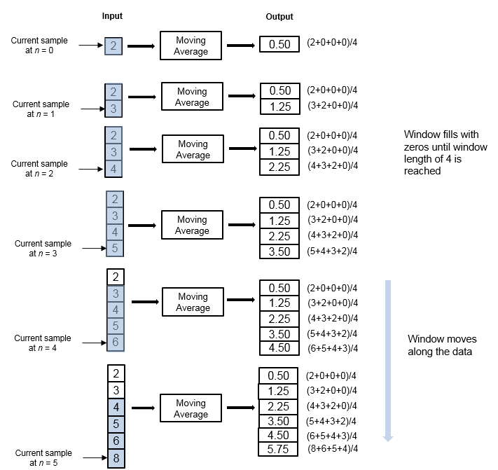
The window is of finite length, making the algorithm a finite impulse response filter. To analyze a statistic over a finite duration of data, use the sliding window method.
Effect of Window Length
The window length defines the length of the data over which the algorithm computes the statistic. The window moves as the new data comes in. If the window is large, the statistic computed is closer to the stationary statistic of the data. For data that does not change rapidly, use a long window to get a smoother statistic. For data that changes fast, use a smaller window.
Effect of Overlap Length
When the overlap length parameter is set to a value less than window length – 1, the algorithm downsamples the output by a factor of hop size (window length – overlap length). In the above example, overlap length is set to 1. In this case, the algorithm produces one output sample at every third input sample starting at n = 3.
Exponential Weighting Method
The exponential weighting method has an infinite impulse response. The algorithm computes a set of weights, and applies these weights to the data samples recursively. As the age of the data increases, the magnitude of the weighting factor decreases exponentially and never reaches zero. In other words, the recent data has more influence on the statistic at the current sample than the older data. Due to the infinite impulse response, the algorithm requires fewer coefficients, making it more suitable for embedded applications.
The value of the forgetting factor determines the rate of change of the weighting factors. A forgetting factor of 0.9 gives more weight to the older data than does a forgetting factor of 0.1. To give more weight to the recent data, move the forgetting factor closer to 0. For detecting small shifts in rapidly varying data, a smaller value (below 0.5) is more suitable. A forgetting factor of 1.0 indicates infinite memory. All the previous samples are given an equal weight. The optimal value for the forgetting factor depends on the data stream. For a given data stream, to compute the optimal value for forgetting factor, see [1].
Consider an example of computing the moving average using the exponential weighting method. The forgetting factor is 0.9.
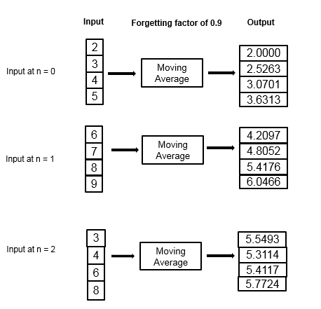
The moving average algorithm updates the weight and computes the moving average recursively for each data sample that comes in by using the following recursive equations.
λ — Forgetting factor.
— Weighting factor applied to the current data sample.
— Current data input sample.
— Moving average at the previous sample.
— Effect of the previous data on the average.
— Moving average at the current sample.
| Data | Weight | Average |
|---|---|---|
| Frame 1 | ||
| 2 | 1. For N = 1, this value is 1. | 2 |
| 3 | 0.9×1+1 = 1.9 | (1–(1/1.9))×2+(1/1.9)×3 = 2.5263 |
| 4 | 0.9×1.9+1 = 2.71 | (1–(1/2.71))×2.52+(1/2.71)×4 = 3.0701 |
| 5 | 0.9×2.71+1 = 3.439 | (1–(1/3.439))×3.07+(1/3.439)×5 = 3.6313 |
| Frame 2 | ||
| 6 | 0.9×3.439+1 = 4.095 | (1–(1/4.095))×3.6313+(1/4.095)×6 = 4.2097 |
| 7 | 0.9×4.095+1 = 4.6855 | (1–(1/4.6855))×4.2097+(1/4.6855)×7 = 4.8052 |
| 8 | 0.9×4.6855+1 = 5.217 | (1–(1/5.217))×4.8052+(1/5.217)×8 = 5.4176 |
| 9 | 0.9×5.217+1 = 5.6953 | (1–(1/5.6953))×5.4176+(1/5.6953)×9 = 6.0466 |
| Frame 3 | ||
| 3 | 0.9×5.6953+1 = 6.1258 | (1–(1/6.1258))×6.0466+(1/6.1258)×3 = 5.5493 |
| 4 | 0.9×6.1258+1 = 6.5132 | (1–(1/6.5132))×5.5493+(1/6.5132)×4 = 5.3114 |
| 6 | 0.9×6.5132+1 = 6.8619 | (1–(1/6.8619))×5.3114+(1/6.8619)×6 = 5.4117 |
| 8 | 0.9×6.8619+1 = 7.1751 | (1–(1/7.1751))×5.4117+(1/7.1751)×8 = 5.7724 |
The moving average algorithm has a state and remembers the data from the previous time step.
For the first sample, when N = 1, the algorithm chooses = 1. For the next sample, the weighting factor is updated and the average is computed using the recursive equations.
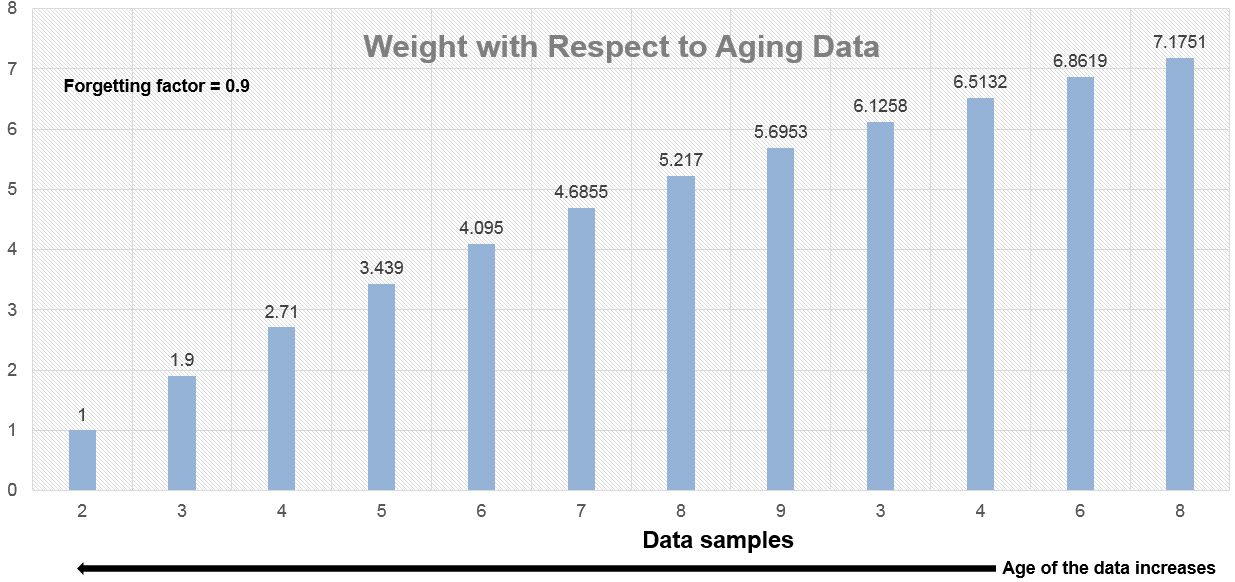
As the age of the data increases, the magnitude of the weighting factor decreases exponentially and never reaches zero. In other words, the recent data has more influence on the current average than the older data.
When the forgetting factor is 0.5, the weights applied to the older data are lower than when the forgetting factor is 0.9.
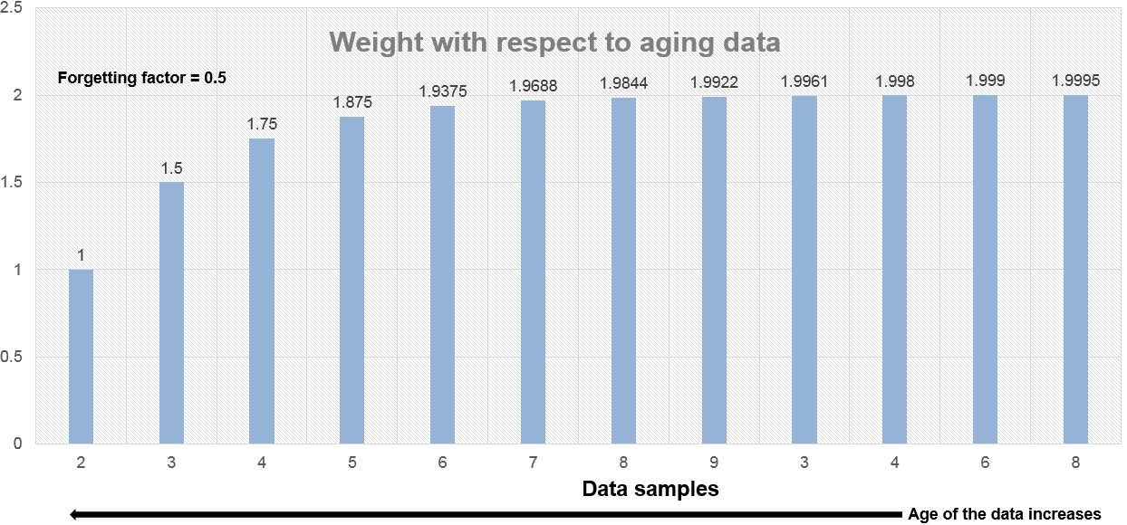
When the forgetting factor is 1, all the data samples are weighed equally. In this case, the exponentially weighted method is the same as the sliding window method with an infinite window length.
When the signal changes rapidly, use a lower forgetting factor. When the forgetting factor is low, the effect of the past data is lesser on the current average. This makes the transient sharper. As an example, consider a rapidly varying noisy step signal.
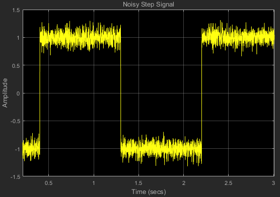
Compute the moving average of this signal using the exponentially weighted method. Compare the performance of the algorithm with forgetting factors 0.8, 0.9, and 0.99.
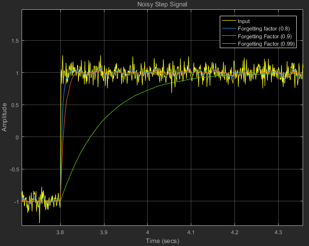
When you zoom in on the plot, you can see that the transient in the moving average is sharp when the forgetting factor is low. This makes it more suitable for data that changes rapidly.
For more information on the moving average algorithm, see the Algorithms section in the dsp.MovingAverage System object™ or
the Moving Average block page.
For more information on other moving statistic algorithms, see the Algorithms section in the respective System object and block pages.
References
[1] Bodenham, Dean. “Adaptive Filtering and Change Detection for Streaming Data.” PH.D. Thesis. Imperial College, London, 2012.