Streaming Signal Statistics
This example shows how to perform statistical measurements on an input data stream using DSP System Toolbox™ functionality available at the MATLAB® command line. Compute the signal statistics minimum, maximum, mean, variance and peak-to-RMS and the signal power spectrum density and plot them.
Introduction
This example computes signal statistics using DSP System Toolbox System objects. These objects handle their states automatically reducing the amount of hand code needed to update states reducing the possible chance of coding errors.
These System objects pre-compute many values used in the processing. This is very useful when you are processing signals of same properties in a loop. For example, in computing an FFT in a spectrum estimation application, the values of sine and cosine can be computed and stored once you know the properties of the input and these values can be reused for subsequent calls. Also the objects check only whether the input properties are of same type as previous inputs in each call.
Initialization
Here you initialize some of the variables used in the code and instantiate the System objects used in your processing. These objects also pre-compute any necessary variables or tables resulting in efficient processing calls later inside a loop.
frameSize = 1024; % Size of one chunk of signal to be processed in one loop
Fs = 48e3;        % Sample rate
numFrames = 100;  % number of frames to process
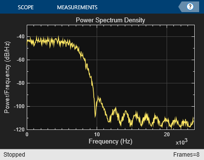
The input signal in this example is white Gaussian noise passed through a lowpass FIR filter. Create the FIR Filter System object™ used to filter the noise signal:
fir = dsp.FIRFilter(Numerator=designLowpassFIR(FilterOrder=32,CutoffFrequency=.3));
Create a Spectrum Estimator System object to estimate the power spectrum density of the input.
spect = dsp.SpectrumEstimator(SampleRate=Fs,...
                              SpectrumType='Power density',...
                              FrequencyRange='onesided',...
                              Window='Kaiser');
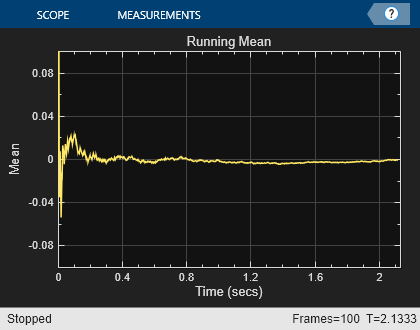
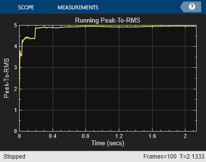
Create System objects to calculate mean, variance, peak-to-RMS, minimum and maximum and set them to running mode. These objects are a subset of statistics System objects available in the product. In running mode, you compute the statistics of the input for its entire length in the past rather than the statistics for just the current input.
runMean       = dsp.MovingAverage(SpecifyWindowLength=false);
runVar        = dsp.MovingVariance(SpecifyWindowLength=false);
runPeaktoRMS  = dsp.PeakToRMS(RunningPeakToRMS=true);
runMin        = dsp.MovingMinimum(SpecifyWindowLength=false);
runMax        = dsp.MovingMaximum(SpecifyWindowLength=false);
Initialize scope System objects, used to visualize statistics and spectrum
meanScope = timescope(SampleRate=Fs,...
                      TimeSpanSource='property',...
                      TimeSpan=numFrames*frameSize/Fs,...
                      Title='Running Mean',...
                      YLabel='Mean',...
                      YLimits=[-0.1 .1],...
                      Position=[43   308   420   330]);
p2rmsScope = timescope(SampleRate=Fs,...
                       TimeSpanSource='property',...
                       TimeSpan=numFrames*frameSize/Fs,...
                       Title='Running Peak-To-RMS',...
                       YLabel='Peak-To-RMS',...
                       YLimits=[0 5],...
                       Position=[480   308   420   330]);
minmaxScope = timescope(SampleRate=Fs,...
                        TimeSpanSource='property', ...
                        TimeSpan=numFrames*frameSize/Fs,...
                        ShowGrid=true,...
                        Title='Signal with Running Minimum and Maximum',...
                        YLabel='Signal Amplitude',...
                        YLimits=[-3 3],...
                        Position=[43   730   422   330]);
spectrumScope = dsp.ArrayPlot(SampleIncrement=.5 * Fs/(frameSize/2 + 1 ),...
                             PlotType='Line',...
                             Title='Power Spectrum Density',...
                             XLabel='Frequency (Hz)',...
                             YLabel='Power/Frequency (dB/Hz)',...
                             YLimits=[-120 -30],...
                             Position=[475 730 420 330]);
Stream Processing Loop
Here you call your processing loop which filters white Gaussian noise and calculates its mean, variance, peak-to-RMS, min, max and spectrum using the System objects.
Note that the System objects are called inside the loop. Since the input data properties do not change, the objects are reused leading to the usage of less memory.
for i=1:numFrames
    % Pass white Gaussian noise through FIR Filter
    sig = fir(randn(frameSize,1));

    % Compute power spectrum density
    ps = spect(sig);

    % The runMean System object keeps track of the information about past
    % samples and gives you the mean value reached until now. The same is
    % true for runMin and runMax System objects.
    meanval  = runMean(sig);
    variance = runVar( sig);
    peak2rms = runPeaktoRMS(sig);
    minimum  = runMin( sig);
    maximum  = runMax(sig);

    % Plot the data you have processed
    minmaxScope([sig,minimum,maximum]);
    spectrumScope(10*log10(ps));
    meanScope(meanval);
    p2rmsScope(peak2rms);
end
release(minmaxScope);

release(spectrumScope);
release(meanScope);
release(p2rmsScope);
Conclusion
You have seen visually that the code involves just calling successive System objects with appropriate input arguments and does not involve maintaining any more variables like indices or counters to compute the statistics. This technique helps in quicker and error free coding. Pre-computation of constant variables inside the objects generally leads to faster processing time.