Train Network on Image and Feature Data

This example shows how to train a network that classifies handwritten digits using both image and feature input data.

Load Training Data

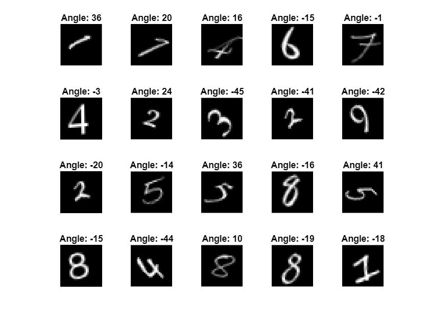
Load the digits images, labels, and clockwise rotation angles.

load DigitsDataTrain

To train a network with multiple inputs using the trainnet function, create a single datastore that contains the training predictors and responses. To convert numeric arrays to datastores, use arrayDatastore. Then, use the combine function to combine them into a single datastore.

dsX1Train = arrayDatastore(XTrain,IterationDimension=4);
dsX2Train = arrayDatastore(anglesTrain);
dsTTrain = arrayDatastore(labelsTrain);
dsTrain = combine(dsX1Train,dsX2Train,dsTTrain);

Display 20 random training images.

numObservationsTrain = numel(labelsTrain);
idx = randperm(numObservationsTrain,20);

figure
tiledlayout("flow");
for i = 1:numel(idx)
    nexttile
    imshow(XTrain(:,:,:,idx(i)))
    title("Angle: " + anglesTrain(idx(i)))
end

Define Network Architecture

Define the following network.

• For the image input, specify an image input layer with size matching the input data.

• For the feature input, specify a feature input layer with size matching the number of input features.

• For the image input branch, specify a convolution, batch normalization, and ReLU layer block, where the convolutional layer has 16 5-by-5 filters.

• To convert the output of the batch normalization layer to a feature vector, include a fully connected layer of size 50.

• To concatenate the output of the first fully connected layer with the feature input, flatten the "SSCB"(spatial, spatial, channel, batch) output of the fully connected layer so that it has format "CB" using a flatten layer.

• Concatenate the output of the flatten layer with the feature input along the first dimension (the channel dimension).

• For classification output, include a fully connected layer with output size matching the number of classes, followed by a softmax layer.

Create an empty neural network.

net = dlnetwork;

Create a layer array containing the main branch of the network and add them to the network.

[h,w,numChannels,numObservations] = size(XTrain);
numFeatures = 1;
classNames = categories(labelsTrain);
numClasses = numel(classNames);

imageInputSize = [h w numChannels];
filterSize = 5;
numFilters = 16;

layers = [
    imageInputLayer(imageInputSize,Normalization="none")
    convolution2dLayer(filterSize,numFilters)
    batchNormalizationLayer
    reluLayer
    fullyConnectedLayer(50)
    flattenLayer
    concatenationLayer(1,2,Name="cat")
    fullyConnectedLayer(numClasses)
    softmaxLayer];

net = addLayers(net,layers);

Add a feature input layer to the network and connect it to the second input of the concatenation layer.

featInput = featureInputLayer(numFeatures,Name="features");
net = addLayers(net,featInput);
net = connectLayers(net,"features","cat/in2");

Visualize the network in a plot.

figure
plot(net)

Specify Training Options

Specify the training options. Choosing among the options requires empirical analysis. To explore different training option configurations by running experiments, you can use the Experiment Manager app.

• Train using the SGDM optimizer.

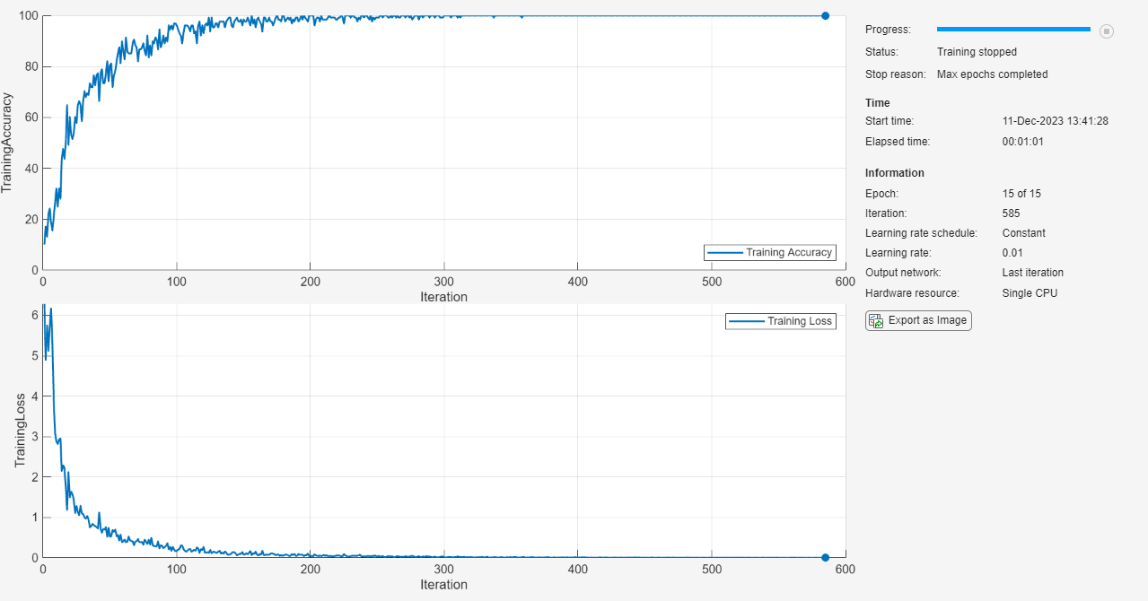
• Train for 15 epochs.

• Train with a learning rate of 0.01.

• Display the training progress in a plot and monitor the accuracy metric.

• Suppress the verbose output.

options = trainingOptions("sgdm", ...
    MaxEpochs=15, ...
    InitialLearnRate=0.01, ...
    Plots="training-progress", ...
    Metrics="accuracy", ...
    Verbose=0);

Train Network

Train the neural network using the trainnet function. For classification, use cross-entropy loss. By default, the trainnet function uses a GPU if one is available. Using a GPU requires a Parallel Computing Toolbox™ license and a supported GPU device. For information on supported devices, see GPU Computing Requirements (Parallel Computing Toolbox). Otherwise, the function uses the CPU. To specify the execution environment, use the ExecutionEnvironment training option.

net = trainnet(dsTrain,net,"crossentropy",options);

Test Network

Load the test data and create a datastore using the same steps as for the training data.

load DigitsDataTest

dsX1Test = arrayDatastore(XTest,IterationDimension=4);
dsX2Test = arrayDatastore(anglesTest);
dsTTest = arrayDatastore(labelsTest);
dsTest = combine(dsX1Test,dsX2Test,dsTTest);

Test the neural network using the testnet function. For single-label classification, evaluate the accuracy. The accuracy is the percentage of correct predictions. By default, the testnet function uses a GPU if one is available. To select the execution environment manually, use the ExecutionEnvironment argument of the testnet function.

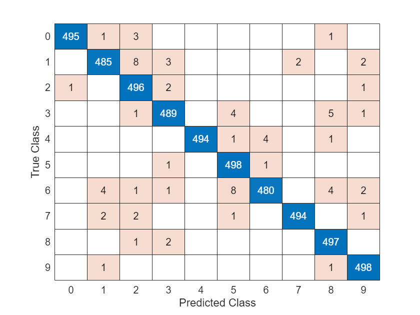
accuracy = testnet(net,dsTest,"accuracy")

accuracy = 98.4000

Visualize the predictions in a confusion chart. Make predictions using the minibatchpredict function and convert the scores to labels using the scores2label function. By default, the minibatchpredict function uses a GPU if one is available.

scores = minibatchpredict(net,XTest,anglesTest);
YTest = scores2label(scores,classNames);

figure
confusionchart(labelsTest,YTest)

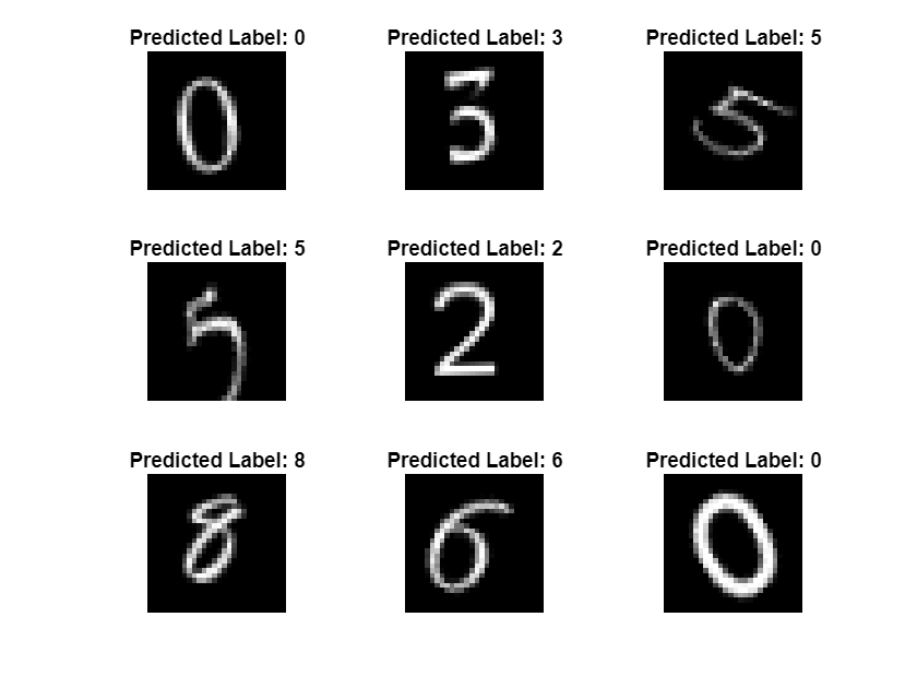
View some of the images with their predictions.

idx = randperm(size(XTest,4),9);
figure
tiledlayout(3,3)
for i = 1:9
    nexttile
    I = XTest(:,:,:,idx(i));
    imshow(I)

    label = string(YTest(idx(i)));
    title("Predicted Label: " + label)
end