Probabilistic Neural Networks

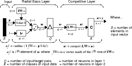
Probabilistic neural networks can be used for classification problems. When an input is presented, the first layer computes distances from the input vector to the training input vectors and produces a vector whose elements indicate how close the input is to a training input. The second layer sums these contributions for each class of inputs to produce as its net output a vector of probabilities. Finally, a compete transfer function on the output of the second layer picks the maximum of these probabilities, and produces a 1 for that class and a 0 for the other classes. The architecture for this system is shown below.

Network Architecture

It is assumed that there are Q input vector/target vector pairs. Each target vector has K elements. One of these elements is 1 and the rest are 0. Thus, each input vector is associated with one of K classes.

The first-layer input weights, IW^1,1 (net.IW{1,1}), are set to the transpose of the matrix formed from the Q training pairs, P'. When an input is presented, the || dist || box produces a vector whose elements indicate how close the input is to the vectors of the training set. These elements are multiplied, element by element, by the bias and sent to the radbas transfer function. An input vector close to a training vector is represented by a number close to 1 in the output vector a¹. If an input is close to several training vectors of a single class, it is represented by several elements of a¹ that are close to 1.

The second-layer weights, LW^1,2 (net.LW{2,1}), are set to the matrix T of target vectors. Each vector has a 1 only in the row associated with that particular class of input, and 0s elsewhere. (Use function ind2vec to create the proper vectors.) The multiplication Ta¹ sums the elements of a¹ due to each of the K input classes. Finally, the second-layer transfer function, compet, produces a 1 corresponding to the largest element of n², and 0s elsewhere. Thus, the network classifies the input vector into a specific K class because that class has the maximum probability of being correct.

Design (newpnn)

You can use the function newpnn to create a PNN. For instance, suppose that seven input vectors and their corresponding targets are

P = [0 0;1 1;0 3;1 4;3 1;4 1;4 3]'

which yields

P =
     0     1     0     1     3     4     4
     0     1     3     4     1     1     3
Tc = [1 1 2 2 3 3 3]

which yields

Tc =
     1     1     2     2     3     3     3

You need a target matrix with 1s in the right places. You can get it with the function ind2vec. It gives a matrix with 0s except at the correct spots. So execute

T = ind2vec(Tc) 

which gives

T =
   (1,1)        1
   (1,2)        1
   (2,3)        1
   (2,4)        1
   (3,5)        1
   (3,6)        1
   (3,7)        1

Now you can create a network and simulate it, using the input P to make sure that it does produce the correct classifications. Use the function vec2ind to convert the output Y into a row Yc to make the classifications clear.

net = newpnn(P,T);
Y = sim(net,P);
Yc = vec2ind(Y)

This produces

Yc =
     1     1     2     2     3     3     3

You might try classifying vectors other than those that were used to design the network. Try to classify the vectors shown below in P2.

P2 = [1 4;0 1;5 2]'
P2 =
     1     0     5
     4     1     2

Can you guess how these vectors will be classified? If you run the simulation and plot the vectors as before, you get

Yc =
     2     1     3

These results look good, for these test vectors were quite close to members of classes 2, 1, and 3, respectively. The network has managed to generalize its operation to properly classify vectors other than those used to design the network.

You might want to try PNN Classification. It shows how to design a PNN, and how the network can successfully classify a vector not used in the design.