Tuning for Multiple Values of Plant Parameters
This example shows how to use Control System Tuner to tune a control system when there are parameter variations in the plant. The control system used in this example is an active suspension of a quarter-car model. The example uses Control System Tuner to tune the system to meet performance objectives when parameters in the plant vary from their nominal values.
Quarter-Car Model and Active Suspension Control
A simple quarter-car model of an active suspension system is shown in Figure 1. The quarter-car model consists of two masses, a car chassis with mass  and a wheel assembly of mass
  . There is a spring
  and damper
  between the masses, which models the passive spring and shock absorber. The tire between the wheel assembly and the road is modeled by the spring
  .
.
Active suspension introduces a force  between the chassis and wheel assembly and allows the designer to balance driving objectives such as passenger comfort and road handling with the use of a feedback controller.
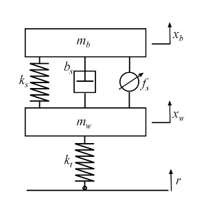
Figure 1: Quarter-car model of active suspension.
Control Architecture
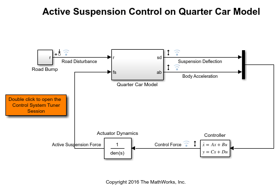
The quarter-car model is implemented using Simscape™. The following Simulink® model contains the quarter-car model with active suspension, controller and actuator dynamics. Its inputs are road disturbance and the force for the active suspension. Its outputs are the suspension deflection and body acceleration. The controller uses these measurements to send a control signal to the actuator that creates the force for active suspension.
mdl = 'rct_suspension.slx';
open_system(mdl)
Control Objectives
The example has the following three control objectives:
Good handling defined from road disturbance to suspension deflection.
User comfort defined from road disturbance to body acceleration.
Reasonable control bandwidth.
The nominal values of the spring constant and damper between the body and the wheel assembly are not exact and due to the imperfections in the materials, these values can be constant but different. Assess the impact on the system control using a variety of parameter values.
Model the road disturbance of magnitude seven centimeters and use a constant weight.
Wroad = ss(0.07);
Define the closed-loop target for handling from road disturbance to suspension deflection as
HandlingTarget = 0.044444 * tf([1/8 1],[1/80 1]);
Define the target for comfort from road disturbance to body acceleration.
ComfortTarget = 0.6667 * tf([1/0.45 1],[1/150 1]);
Limit the control bandwidth by the weight function from road disturbance to the control signal.
Wact = tf(0.1684*[1 500],[1 50]);
For more information on selecting the closed-loop targets and the weight function, see Robust Control of Active Suspension (Robust Control Toolbox).
Controller Tuning
To open a Control System Tuner session for active suspension control, in the Simulink model, Double click to the orange block. Tuned block is set to the second order Controller and three tuning goals are defined to achieve the handling, comfort and control bandwidth as described above. In order to see the performance of the tuning, the step responses from road disturbance to suspension deflection, the body acceleration and the control force are plotted.
Handling, comfort, and control bandwidth goals are defined as gain limits, HandlingTarget/Wroad, ComfortTarget/Wroad and Wact/Wroad. All gain functions are divided by Wroad to incorporate the road disturbance.
The open-loop system with zero controller violates the handling goal and results in highly oscillatory behavior for both suspension deflection and body acceleration with long settling time.
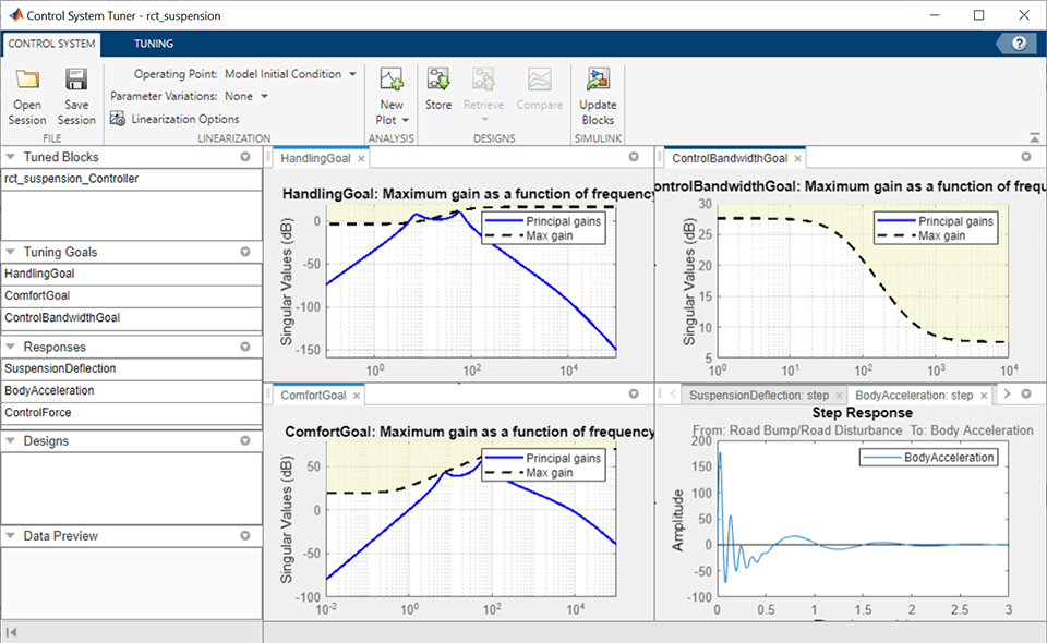
Figure 2: Control System Tuner with Session File.
To tune the controller using Control System Tuner, on the Tuning tab, click Tune. As shown in Figure 3, this design satisfies the tuning goals and the responses are less oscillatory and converges quickly to zero.
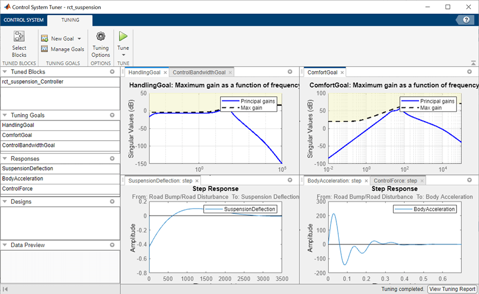
Figure 3: Control System Tuner after tuning.
Controller Tuning for Multiple Parameter Values
Now, try to tune the controller for multiple parameter values. The default value for car chassis of mass is 300 kg. Vary the mass to 100 kg, 200 kg and 300 kg for different operation conditions.
In order to vary these parameters in Control System Tuner, on the Control System tab, under Parameter Variations, select Select parameters to Vary. Define the parameters in the dialog box that opens.
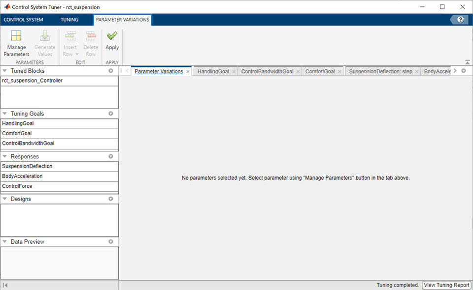
Figure 4: Defining parameter variations.
On the Parameter Variations tab, click Manage Parameters. In the Select model variables dialog box, select Mb.
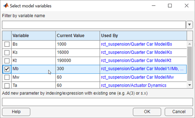
Figure 5: Select a parameter to vary from the model.
Now, the parameter Mb is added with default values in the parameter variations table.
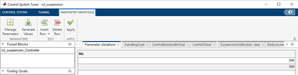
Figure 6: Parameter variations table with default values.
To generate variations quickly, click Generate Values. In the Generate Parameter Values dialog box, define values 100, 200, 300 for Mb, and click Overwrite.
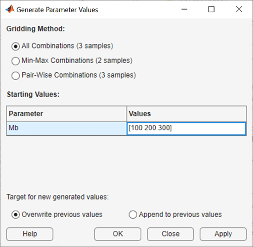
Figure 7: Generate values window.
All values are populated in the parameter variations table. To set the parameter variations to Control System Tuner, click Apply.
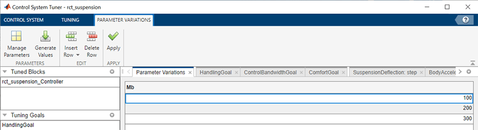
Figure 8: Parameter variations table with updated values.
Multiple lines appear in the tuning goal and response plots due to the varying parameters. The controller obtained for these nominal parameter values results in an unstable closed-loop system.
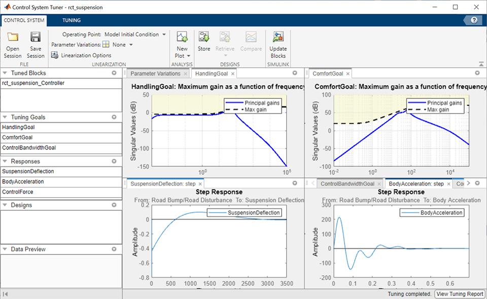
Figure 9: Control System Tuner with multiple parameter variations.
Tune the controller to satisfy the handling, comfort, and control bandwidth objectives by clicking Tune in Tuning tab. The tuning algorithm tries to satisfy these objectives for the nominal parameters and for all parameter variations. This is a challenging task in contrast to nominal design as shown in Figure 10.
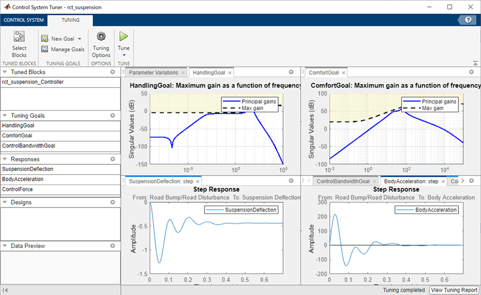
Figure 10: Control System Tuner with multiple parameter variations (Tuned).
Control System Tuner tunes the controller parameters for the linearized control system. To examine the performance of the tuned parameters on the Simulink model, update the controller in the Simulink model by clicking Update Blocks on the Control System tab.
Simulate the model for each of the parameter variations. Then, using the Simulation Data Inspector, examine the results for all simulations. The results are shown in Figure 11. For all three parameter variations, the controller tries to minimize the suspension deflection and body acceleration with minimal control effort.
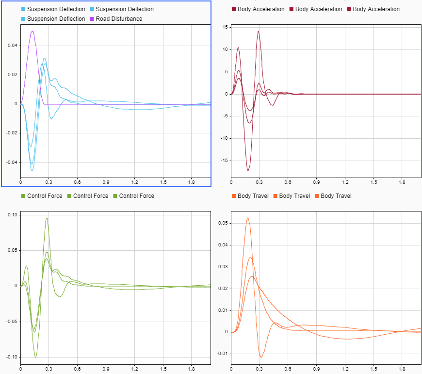
Figure 11: Controller performance on the Simulink model.