disconeStrip

Create stripped discone antenna

Since R2020b

Description

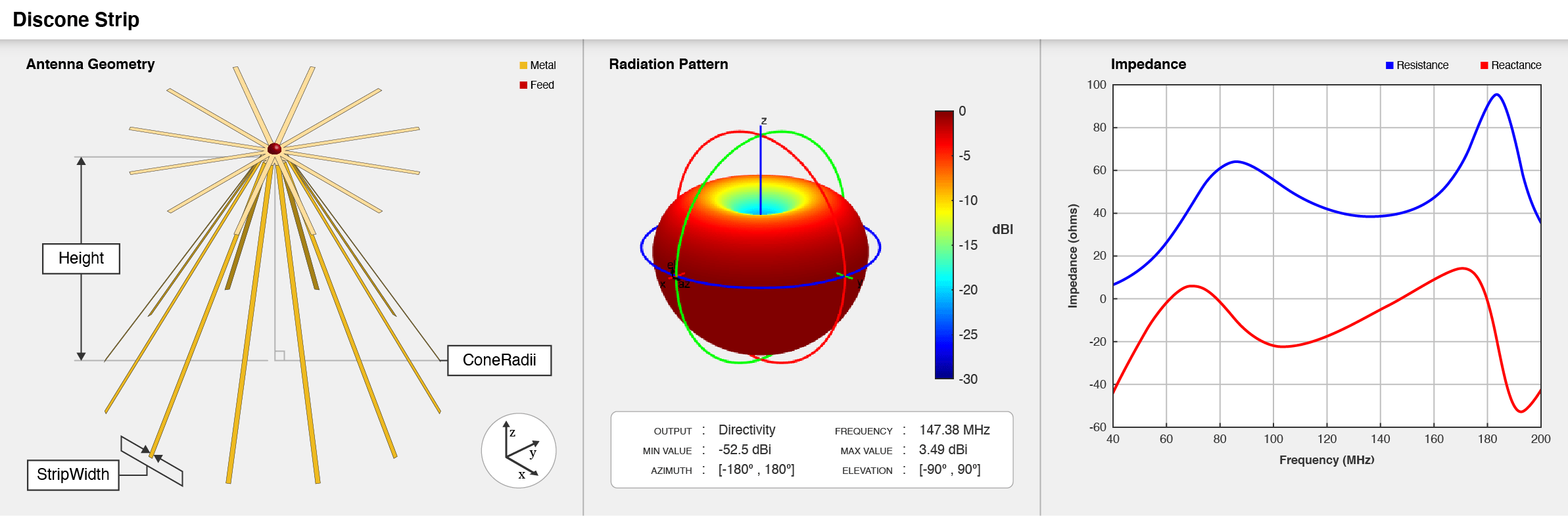
The default disconeStrip object creates a stripped discone antenna resonating around 147.38 MHz. The stripped discone antenna is an approximation to a solid discone antenna, where the cone and the disc are replaced with strips. The stripped discone antennas are lighter in weight and suited for applications in high frequency (HF) and very high frequency (VHF) bands.

Creation

Syntax

ds = disconeStrip

ds = disconeStrip(Name=Value)

Description

ds = disconeStrip creates a strip discone antenna with default property values. The default dimensions are chosen for an operating frequency of around 147.38 MHz. The default stripped discone antenna has a feed point at the center of the disc.

ds = disconeStrip(Name=Value) sets properties using one or more name-value arguments. Name is the property name and Value is the corresponding value. You can specify several name-value arguments in any order as Name1=Value1,...,NameN=ValueN. Properties that you do not specify, retain their default values.

For example, ds = disconeStrip(NumStrips=8) creates a discone strip antenna with eight strips and default values for other properties.

Properties

NumStrips — Number of strips

12 (default) | positive scalar in the range [6, 64]

Number of strips to form the cone and the disc, specified as a positive scalar in the range [6, 64]. The number of strips can be increased to increase the impedance bandwidth of the disconeStrip object.

Example: 8

Data Types: double

StripWidth — Width of strip

20e-3 (default) | scalar

Width of each strip in the strip discone antenna, specified as a scalar in meters.

Example: 10e-3

Data Types: double

Height — Vertical height between broad and narrow diameter of cone

1.308 (default) | positive scalar

Vertical height between the maximum or broad diameter and the minimum or narrow diameter of the cone, specified as a positive scalar in meters. The vertical height can be decreased to increase the operating frequency.

Example: 1.59

Data Types: double

ConeRadii — Narrow and broad radii of cone

[65e-3 810e-3] (default) | two-element vector

Narrow and broad radii of the cone, specified as a two-element vector in meters. In the two element vector, the first element specifies the narrow or minimum radius and second element specifies the broad or maximum radius of the cone. The radii of the cone can be decreased to increase the operating frequency and high-frequency input impedance.

Example: [63e-3 840e-3]

Data Types: double

DiscRadius — Radius of disc

700e-3 (default) | scalar

Radius of the disc, specified as a scalar in meters. The radius of the disc can be decreased to increase the operating frequency and it can be increased to increase the low-frequency input impedance.

Note

DiscRadius must be smaller than the ConeRadii.

Example: 900e-3

Data Types: double

FeedHeight — Gap between cone and disc

30e-3 (default) | positive scalar

Gap between the cone and the disc, specified as a positive scalar in meters. This gap represents height of the field and the gap can be decreased to increase the high-frequency input impedance.

Example: 34e-3

Data Types: double

FeedWidth — Diameter of feed

20e-3 (default) | positive scalar

Diameter of the feed, specified as a positive scalar in meters.

Example: 25e-3

Data Types: double

Conductor — Type of metal

metal("PEC") (default) | metal object

Type of the metal used as a conductor, specified as a metal object. You can choose any metal from the MetalCatalog or specify a metal of your choice. For more information on metal conductor meshing, see Meshing.

Example: metal("Copper")

Load — Lumped elements

[1x1 lumpedElement] (default) | lumpedElement object

Lumped elements added to the antenna feed, specified as a lumpedElement object. You can add a load anywhere on the surface of the antenna. By default, the load is at the feed.

Example: Load=lumpedElement(Impedance=75)

Example: antenna.Load = lumpedElement(Impedance=75)

Tilt — Tilt angle of antenna

0 (default) | scalar | vector

Tilt angle of the antenna in degrees, specified as a scalar or vector. For more information, see Rotate Antennas and Arrays.

Example: 90

Example: Tilt=[90 90],TiltAxis=[0 1 0;0 1 1] tilts the antenna at 90 degrees about the two axes defined by the vectors.

Data Types: double

TiltAxis — Tilt axis of antenna

[1 0 0] (default) | three-element vector | 2-by-3 matrix | "X" | "Y" | "Z"

Tilt axis of the antenna, specified as one of these values:

• Three-element vector of Cartesian coordinates in meters. In this case, each coordinate in the vector starts at the origin and lies along the specified points on the x-, y-, and z-axes.

• Two points in space, specified as a 2-by-3 matrix corresponding to two three-element vectors of Cartesian coordinates. In this case, the antenna rotates around the line joining the two points.

• "x", "y", or "z" to describe a rotation about the x-, y-, or z-axis, respectively.

For more information, see Rotate Antennas and Arrays.

Example: [0 1 0]

Example: [0 0 0;0 1 0]

Example: "Z"

Data Types: double | string

Object Functions

axialRatio	Calculate and plot axial ratio of antenna or array
bandwidth	Calculate and plot absolute bandwidth of antenna or array
beamwidth	Beamwidth of antenna
charge	Charge distribution on antenna or array surface
coneangle2size	Calculates equivalent cone height, broad radius, and narrow radius
current	Current distribution on antenna or array surface
design	Design prototype antenna or arrays for resonance around specified frequency or create AI-based antenna from antenna catalog objects
efficiency	Calculate and plot radiation efficiency of antenna or array
EHfields	Electric and magnetic fields of antennas or embedded electric and magnetic fields of antenna element in arrays
feedCurrent	Calculate current at feed for antenna or array
impedance	Calculate and plot input impedance of antenna or scan impedance of array
info	Display information about antenna, array, or platform
memoryEstimate	Estimate memory required to solve antenna or array mesh
mesh	Mesh properties of metal, dielectric antenna, or array structure
meshconfig	Change meshing mode of antenna, array, custom antenna, custom array, or custom geometry
msiwrite	Write antenna or array analysis data to MSI planet file
optimize	Optimize antenna or array using SADEA optimizer
pattern	Plot radiation pattern and phase of antenna or array or embedded pattern of antenna element in array
patternAzimuth	Azimuth plane radiation pattern of antenna or array
patternElevation	Elevation plane radiation pattern of antenna or array
peakRadiation	Calculate and mark maximum radiation points of antenna or array on radiation pattern
rcs	Calculate and plot monostatic and bistatic radar cross section (RCS) of platform, antenna, or array
resonantFrequency	Calculate and plot resonant frequency of antenna
returnLoss	Calculate and plot return loss of antenna or scan return loss of array
show	Display antenna, array structures, shapes, or platform
sparameters	Calculate S-parameters for antenna or array
stlwrite	Write mesh information to STL file
vswr	Calculate and plot voltage standing wave ratio (VSWR) of antenna or array element

Examples

Design Strip Discone Antenna with Default Properties

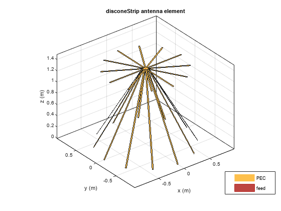
Create and view a strip discone antenna with default properties.

ant = disconeStrip;
show(ant)

Plot the radiation pattern of the antenna at 147.38 MHz.

pattern(ant, 147.38e6)

Create Strip Discone Antenna and Plot S-Parameters

Create and view a strip discone antenna object with the specified properties.

ant = disconeStrip(Height=92e-3, ConeRadii=[5.5e-3 53e-3], DiscRadius=37e-3, NumStrip=16,...
    StripWidth=1e-3, FeedWidth=0.5e-3, FeedHeight=2.2e-3);
show(ant)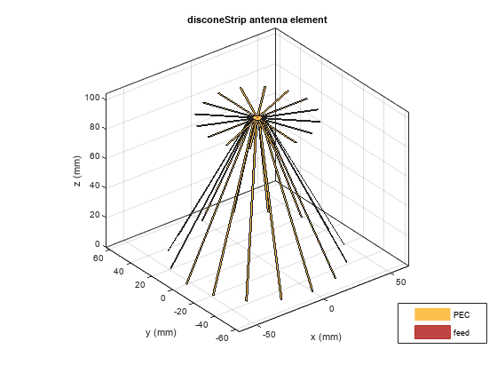

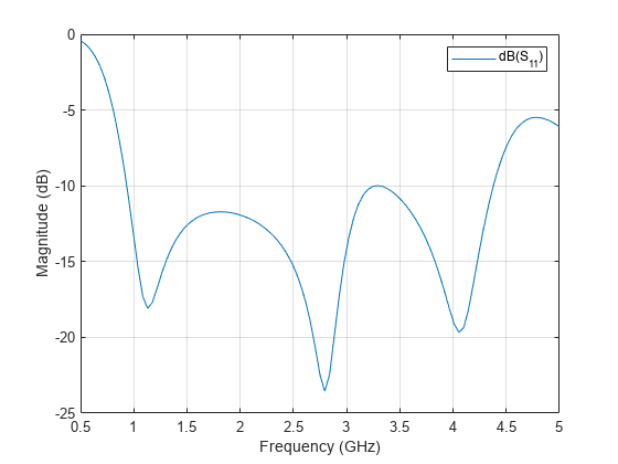
Plot the S-Parameters of the antenna over the frequency span of 500 MHz to 5 GHz.

s = sparameters(ant,linspace(500e6,5e9,101));
figure
rfplot(s)

More About

Parametric Analysis Guidelines

To understand how the properties of the disconeStrip antenna object influence the antenna design, use the following parametric analysis guidelines.

• To increase the operating frequency, decrease the dimensions of the disconeStrip antenna object using the ConeRadii, DiscRadius, and Height properties.

• To increase the impedance bandwidth, increase the number of strips in the disconeStrip antenna object using the NumStrips property.

• To improve high-frequency input impedance, decrease the cone radii and feed height of the antenna using the ConeRadii and the FeedHeight properties.

• To increase low frequency input impedance, increase the radius of the disc using the DiscRadius property.

References

[1] Khumanthem.T., C.Sairam, S.D.Ahirwar and M.Balachary. ''Compact Discone Antenna with Small Form Factor in VHF Band'' EWCI, 2014.

[2] Ki-Hak Kim, Jin-U Kim, and Seong-Ook Park. “An Ultrawide-Band Double Discone Antenna with the Tapered Cylindrical Wires.” IEEE Transactions on Antennas and Propagation 53, no. 10 (October 2005): 3403–6. https://doi.org/10.1109/TAP.2005.856036.

[3] Tai C-T. and S. A. Long. ''Dipoles and Monopoles'' in Antenna Engineering Handbook, 4th ed., J. L. Volakis (Ed.), McGraw-Hill, 2007.

[4] McDonald, James L., and Dejan S. Filipovic. “On the Bandwidth of Monocone Antennas.” IEEE Transactions on Antennas and Propagation 56, no. 4 (April 2008): 1196–1201. https://doi.org/10.1109/TAP.2008.919226.

Version History

Introduced in R2020b