synthesizeTabularData
Synthesize tabular data using binning-based or SMOTE-based synthesizer
Since R2024b
Syntax
Description
syntheticX = synthesizeTabularData(synthesizer,n)n observations of synthetic data using a trained synthesizer.
The function uses the information in synthesizer to return the
synthetic data syntheticX.
[
additionally returns the synthetic class labels syntheticX,syntheticY] = synthesizeTabularData(synthesizer,n)syntheticY. To return
nonempty syntheticY, you must create synthesizer
using existing class labels as a separate variable (Y). (since R2026a)
___ = synthesizeTabularData(___,
specifies options using one or more name-value arguments in addition to any of the input
argument combinations in the previous syntaxes. For example, you can specify the class for
which to generate observations and the options for computing in parallel.Name=Value)
Examples
Use existing training data to create a binningTabularSynthesizer object. Then, synthesize data using the synthesizeTabularData object function. Train a model using the existing training data, and then train the same type of model using the synthetic data. Compare the performance of the two models using test data.
Load the carbig data set, which contains measurements of cars made in the 1970s and early 1980s. Create a table containing the predictor variables Acceleration, Displacement, and so on, as well as the response variable MPG.
load carbig
tbl = table(Acceleration,Cylinders,Displacement,Horsepower, ...
    Model_Year,Origin,MPG,Weight);
Remove rows of tbl where the table has missing values.
tbl = rmmissing(tbl);
Partition the data into training and test sets. Use approximately 60% of the observations for model training and synthesizing new data, and 40% of the observations for model testing. Use cvpartition to partition the data.
rng("default")
cv = cvpartition(size(tbl,1),"Holdout",0.4);
trainTbl = tbl(training(cv),:);
testTbl = tbl(test(cv),:);
Create a binningTabularSynthesizer object by using the trainTbl data set. The binningTabularSynthesizer function uses binning techniques to learn the distribution of the multivariate data set. Use 20 equal-width bins for each continuous variable. Specify the Cylinders and Model_Year variables as discrete numeric variables.
synthesizer = binningTabularSynthesizer(trainTbl, ...
    BinMethod="equal-width",NumBins=20, ...
    DiscreteNumericVariables=["Cylinders","Model_Year"])
synthesizer =
  binningTabularSynthesizer

               VariableNames: ["Acceleration"    "Cylinders"    "Displacement"    "Horsepower"    "Model_Year"    "Origin"    "MPG"    "Weight"]
        CategoricalVariables: 6
    DiscreteNumericVariables: [2 5]
             BinnedVariables: [1 3 4 7 8]
                   BinMethod: "equal-width"
                     NumBins: [20 20 20 20 20]
                    BinEdges: {[21×1 double]  [21×1 double]  [21×1 double]  [21×1 double]  [21×1 double]}
             NumObservations: 236


  Properties, Methods
synthesizer is a binningTabularSynthesizer object with five binned variables. Each binned variable has the same number of bins.
Synthesize new data by using synthesizer. Specify to generate 1000 observations.
syntheticTbl = synthesizeTabularData(synthesizer,1000);
The synthesizeTabularData object function uses the data distribution information stored in synthesizer to generate syntheticTbl.
To visualize the difference between the existing data and synthetic data, you can use the detectdrift function. The function uses permutation testing to detect drift between trainTbl and syntheticTbl.
dd = detectdrift(trainTbl,syntheticTbl);
dd is a DriftDiagnostics object with plotEmpiricalCDF and plotHistogram object functions for visualization.
For continuous variables, use the plotEmpiricalCDF function to see the difference between the empirical cumulative distribution function (ecdf) of the values in trainTbl and the ecdf of the values in syntheticTbl.
continuousVariable ="Displacement"; plotEmpiricalCDF(dd,Variable=continuousVariable) legend(["Real data","Synthetic data"])
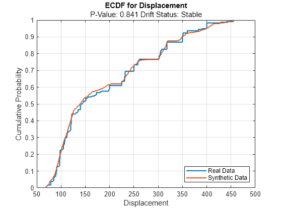
For the Displacement predictor, the ecdf plot for the existing values (in blue) matches the ecdf plot for the synthetic values (in red) fairly well.
For discrete variables, use the plotHistogram function to see the difference between the histogram of the values in trainTbl and the histogram of the values in syntheticTbl.
discreteVariable ="Model_Year"; plotHistogram(dd,Variable=discreteVariable) legend(["Real data","Synthetic data"])
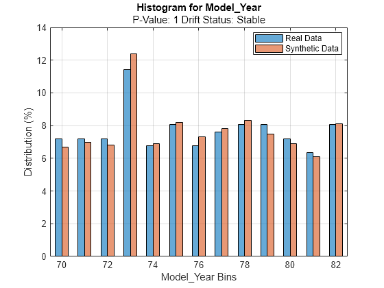
For the Model_Year predictor, the histogram for the existing values (in blue) matches the histogram for the synthetic values (in red) fairly well.
Train a bagged ensemble of trees using the original training data trainTbl. Specify MPG as the response variable. Then, train the same kind of regression model using the synthetic data syntheticTbl.
originalMdl = fitrensemble(trainTbl,"MPG",Method="Bag");
newMdl = fitrensemble(syntheticTbl,"MPG",Method="Bag");
Evaluate the performance of the two models on the test set by computing the test mean squared error (MSE). Smaller MSE values indicate better performance.
originalMSE = loss(originalMdl,testTbl)
originalMSE =
7.0784
newMSE = loss(newMdl,testTbl)
newMSE =
6.1031
The model trained on the synthetic data performs slightly better on the test data.
Use existing training data to create a smoteTabularSynthesizer object. Then, synthesize data using the synthesizeTabularData object function. Train a model using the existing training data, and then train the same type of model using both the existing training data and the synthetic data. Compare the performance of the two models using test data.
Load the carbig data set, which contains measurements of cars made in the 1970s and early 1980s. Categorize the cars based on whether they were made in Europe.
load carbig
Origin = categorical(cellstr(Origin));
Origin = mergecats(Origin,["France","Germany", ...
    "Sweden","Italy","England"],"Europe");
Origin = mergecats(Origin,["USA","Japan"],"NotEurope");
tabulate(Origin)
      Value    Count   Percent
     Europe       73     17.98%
  NotEurope      333     82.02%
The data is imbalanced, with only about 18% of cars originating in Europe.
Create a table containing the variables Acceleration, Displacement, and so on, as well as the response variable Origin. Remove rows of cars where the table has missing values.
cars = table(Acceleration,Displacement,Horsepower, ...
    MPG,Weight,Origin);
cars = rmmissing(cars);
Partition the data into training and test sets. Use approximately 50% of the observations for model training and synthesizing new data, and 50% of the observations for model testing. Use stratified partitioning so that approximately the same ratio of European to non-European cars exists in both the training and test sets.
rng("default")
cv = cvpartition(cars.Origin,Holdout=0.5);
trainCars = cars(training(cv),:);
testCars = cars(test(cv),:);
Create a smoteTabularSynthesizer object using the trainCars data set. Specify Origin as the class labels variable.
synthesizer = smoteTabularSynthesizer(trainCars,"Origin")synthesizer =
smoteTabularSynthesizer
VariableNames: ["Acceleration" "Displacement" "Horsepower" "MPG" "Weight"]
ClassNames: [Europe NotEurope]
NumNeighbors: [5 5]
Distance: "seuclidean"
NumObservations: [34 162]
Properties, Methods
synthesizer is a smoteTabularSynthesizer object with two classes (Europe and NotEurope).
Synthesize new data by using synthesizer. Specify to generate 40 observations belonging to the class of European cars only.
syntheticCars = synthesizeTabularData(synthesizer,40,ClassNames="Europe"); The synthesizeTabularData object function uses the information stored in synthesizer to generate syntheticCars.
To visualize the difference between the existing European car data and the synthetic European car data, you can use the detectdrift function. Filter the trainCars data to include European car data only. The detectdrift function uses permutation testing to detect drift between europeanCars and syntheticCars.
europeanCars = trainCars(trainCars.Origin=="Europe",:);

dd = detectdrift(europeanCars,syntheticCars);
dd is a DriftDiagnostics object with a plotEmpiricalCDF object function for visualization.
For the continuous variables, use the plotEmpiricalCDF function to see the difference between the empirical cumulative distribution function (ecdf) of the values in europeanCars and the ecdf of the values in syntheticCars.
continuousVariable ="Acceleration"; plotEmpiricalCDF(dd,Variable=continuousVariable) legend(["Real data","Synthetic data"])
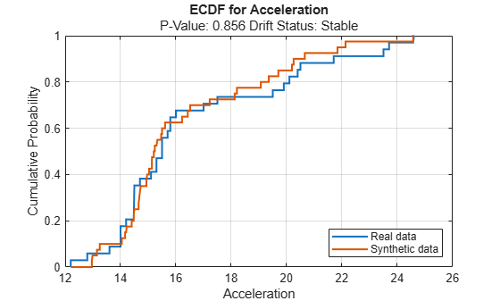
For the Acceleration predictor, the ecdf plot for the existing values (in blue) matches the ecdf plot for the synthetic values (in red) fairly well.
Train an SVM classifier using the original training data trainCars. Specify Origin as the response variable, and standardize the predictors before training. Then, train the same kind of classifier using both the original data and the synthetic data (syntheticCars).
originalMdl = fitcsvm(trainCars,"Origin",Standardize=true);
newMdl = fitcsvm([trainCars;syntheticCars],"Origin",Standardize=true);
Evaluate the performance of the two models on the test set using confusion matrices.
originalPredictions = predict(originalMdl,testCars);
newPredictions = predict(newMdl,testCars);

tiledlayout(1,2)
nexttile
confusionchart(testCars.Origin,originalPredictions)
title("Original Model")
nexttile
confusionchart(testCars.Origin,newPredictions)
title("New Model")
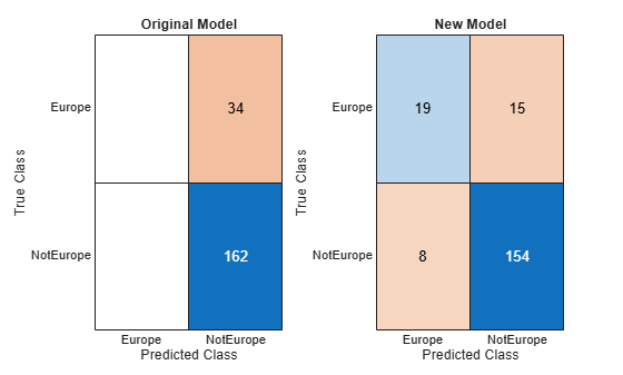
The model trained on the original data classifies all test observations as non-European cars. The model trained on the original and synthetic data has greater accuracy than the other model and correctly classifies the majority of European cars in the test set.
Evaluate data synthesized from an existing data set. Compare the existing and synthetic data sets to determine the similarity between the two multivariate data distributions.
Load the sample file fisheriris.csv, which contains iris data including sepal length, sepal width, petal width, and species type. Read the file into a table, and then convert the Species variable into a categorical variable. Print a summary of the variables in the table.
fisheriris = readtable("fisheriris.csv");
fisheriris.Species = categorical(fisheriris.Species);
summary(fisheriris)
fisheriris: 150×5 table
Variables:
SepalLength: double
SepalWidth: double
PetalLength: double
PetalWidth: double
Species: categorical (3 categories)
Statistics for applicable variables:
NumMissing Min Median Max Mean Std
SepalLength 0 4.3000 5.8000 7.9000 5.8433 0.8281
SepalWidth 0 2 3 4.4000 3.0573 0.4359
PetalLength 0 1 4.3500 6.9000 3.7580 1.7653
PetalWidth 0 0.1000 1.3000 2.5000 1.1993 0.7622
Species 0
The summary display includes statistics for each variable. For example, the sepal length values range from 4.3 to 7.9, with a median of 5.8.
Create 150 new observations from the data in fisheriris. First, create an object by using the binningTabularSynthesizer function. Then, synthesize the data by using the synthesizeTabularData object function. Print a summary of the variables in the new syntheticData data set.
rng(0,"twister") % For reproducibility
synthesizer = binningTabularSynthesizer(fisheriris);
syntheticData = synthesizeTabularData(synthesizer,150);
summary(syntheticData)
syntheticData: 150×5 table

Variables:

    SepalLength: double
    SepalWidth: double
    PetalLength: double
    PetalWidth: double
    Species: categorical (3 categories)

Statistics for applicable variables:

                   NumMissing       Min          Median         Max           Mean          Std

    SepalLength        0           4.3079        5.7174        7.6399        5.8280        0.8576
    SepalWidth         0           2.0236        3.0336        4.2866        3.0819        0.4572
    PetalLength        0           1.0010        4.4453        6.8538        3.6572        1.8192
    PetalWidth         0           0.1002        1.3502        2.4759        1.1719        0.7597
    Species            0
You can compare the variable statistics for syntheticData to the variable statistics for fisheriris. For example, the sepal length values in the synthetic data set range from approximately 4.3 to 7.6, with a median of 5.7. These statistics are similar to the statistics in the fisheriris data set.
Visually compare the observations in fisheriris and syntheticData by using scatter plots. Each point corresponds to an observation. The point color indicates the species of the corresponding iris.
tiledlayout(1,2)
nexttile
gscatter(fisheriris.SepalLength,fisheriris.PetalLength,fisheriris.Species)
xlabel("Sepal Length")
ylabel("Petal Length")
title("Existing Data")
nexttile
gscatter(syntheticData.SepalLength,syntheticData.PetalLength,syntheticData.Species)
xlabel("Sepal Length")
ylabel("Petal Length")
title("Synthetic Data")
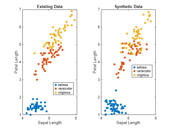
The scatter plots indicate that the existing data set and the synthetic data set have similar characteristics.
Compare the existing and synthetic data sets by using the mmdtest function. The function performs a two-sample hypothesis test for the null hypothesis that the data sets come from the same distribution.
[mmd2,p,h] = mmdtest(fisheriris,syntheticData)
mmd2 =
0.0020
p =
0.9600
h =
0
The returned value of h = 0 indicates that mmdtest fails to reject the null hypothesis that the data sets come from different distributions at the significance level of 5%. As with other hypothesis tests, this result does not guarantee that the null hypothesis is true. That is, the data sets do not necessarily come from the same distribution, but the low mmd2 value (square maximum mean discrepancy) and the high p-value indicate that the distributions of the real and synthetic data sets are similar.
Input Arguments
Trained synthesizer, specified as a binningTabularSynthesizer or smoteTabularSynthesizer object.
Number of synthetic data observations to generate, specified as a positive integer scalar or a two-element positive integer vector.
To generate synthetic data for two classes,
you can specify n as a two-element vector. Each element indicates
the number of observations to generate for the corresponding class in
ClassNames. If you specify n as a scalar,
then the software generates synthetic observations for the two classes with
approximately the same proportion found in
synthesizer.NumObservations. (since R2026a)
Example: 100
Data Types: single | double
Name-Value Arguments
Specify optional pairs of arguments as
Name1=Value1,...,NameN=ValueN, where Name is
the argument name and Value is the corresponding value.
Name-value arguments must appear after other arguments, but the order of the
pairs does not matter.
Example: synthesizeTabularData(synthesizer,10,ClassNames="b",Options=statset(UseParallel=true))
specifies to generate 10 synthetic observations for class "b" in
parallel.
Since R2026a
Names of the classes for which to generate synthetic data, specified as a numeric, categorical, or logical vector; a character or string array; or a cell array of character vectors.
You can use ClassNames to:
Specify the order of the classes.
Select a class for generating synthetic data. For example, suppose that the set of distinct class labels is
["b","g"]. To generate synthetic observations from class"g"only, specifyClassNames="g".
The default value for ClassNames is the ordered set of
distinct class labels in the class labels variable used to create
synthesizer.
Example: ClassNames=["g","b"]
Data Types: single | double | logical | char | string | cell | categorical
Options for computing in parallel and setting random streams, specified as a
structure. Create the Options structure using statset. This table lists the option fields and their
values.
| Field Name | Value | Default |
|---|---|---|
UseParallel | Set this value to true to run computations in
parallel. | false |
UseSubstreams | Set this value to To compute
reproducibly, set | false |
Streams | Specify this value as a RandStream object or
cell array of such objects. Use a single object except when the
UseParallel value is true
and the UseSubstreams value is
false. In that case, use a cell array that
has the same size as the parallel pool. | If you do not specify Streams, then
synthesizeTabularData uses the default stream or
streams. |
Note
You need Parallel Computing Toolbox™ to run computations in parallel.
Example: Options=statset(UseParallel=true,UseSubstreams=true,Streams=RandStream("mlfg6331_64"))
Data Types: struct
Output Arguments
Synthetic data set, returned as a numeric matrix or a table.
syntheticX has the same data type as the data used to create
synthesizer.
If you used Yname to
create synthesizer, then the last column of the
syntheticX table contains the class labels for the synthetic data
set. (since R2026a)
Since R2026a
Synthetic class labels, returned as a numeric, categorical, or logical vector; a
character or string array; or a cell array of character vectors.
syntheticY has the same data type as the class labels used to
create synthesizer.
Algorithms
When you use a binning technique, the process for estimating the multivariate data
distribution includes computing the probability of each unique row in the one-hot encoded
data set (after binning continuous variables). The
synthesizeTabularData function uses this estimated multivariate
data distribution to generate synthetic observations. The function performs these steps:
Use the previously computed probabilities to sample with replacement
nrows from the unique rows in the encoded data set.Decode the sampled data to obtain the bin indices (for continuous variables) and categories (for discrete variables).
For the binned variables, uniformly sample from within the bin edges to obtain continuous values. If you use equiprobable binning (
BinMethod) and the extreme bin widths are greater than 1.5 times the median of the nonextreme bin widths, then the function samples from the cumulative distribution function (cdf) in the extreme bins.
SMOTE (synthetic minority oversampling technique) is a technique for generating synthetic data when you have an imbalanced data set, that is, when the number of observations is not uniform across the response classes.
Assume the data set X has two classes, where class kbig has many more observations than class ksmall. If the data set X has only one class, then assume
all observations belong to ksmall. When you use SMOTE, the synthesizeTabularData
function generates each new ksmall observation in the following way:
Randomly select an observation x in ksmall.
In the data set, find the
NumNeighbors-nearest neighbors of x that also belong to ksmall.Randomly select one of the nearest neighbors .
For each continuous predictor p, set the predictor value of the new observation to , where xp is the predictor value of the original observation x, is the predictor value of the nearest neighbor , and r is a random value in (0,1) as selected by the
randfunction.For the categorical predictors q1, …, qm, set the predictor values of the new observation to the mode of the vector of predictor values among the
NumNeighbors-nearest neighbors of x. In the case of a tie, choose a vector at random.
The function follows the same process to generate observations in class kbig. The number of synthetic observations generated depends on
n (the input argument of
synthesizeTabularData).
References
[1] Chawla, Nitesh V., Kevin W. Bowyer, Lawrence O. Hall, and W. Philip Kegelmeyer. "SMOTE: Synthetic Minority Over-sampling Technique." Journal of Artificial Intelligence Research 16 (2002): 321-357.
Extended Capabilities
To run in parallel, specify the Options name-value argument in the call to
this function and set the UseParallel field of the
options structure to true using
statset:
Options=statset(UseParallel=true)
For more information about parallel computing, see Run MATLAB Functions with Automatic Parallel Support (Parallel Computing Toolbox).
Version History
Introduced in R2024bYou can use the synthetic minority oversampling technique (SMOTE) algorithm to generate synthetic data for binary classification. Using SMOTE can be helpful when you have imbalanced data, that is, when one class contains many more observations than the other.
First, create a smoteTabularSynthesizer object. You can adjust parameters of the SMOTE technique
by using the NumNeighbors, Distance, and
CacheSize name-value arguments. Then call the synthesizeTabularData object function to synthesize data using the
object.
Regardless of whether you use a binningTabularSynthesizer or smoteTabularSynthesizer object,
the synthesizeTabularData function can return synthetic observations
for one or two classes. Use the Yname or Y input
argument when you create the object, and the ClassNames name-value
argument when you call synthesizeTabularData.
MATLAB Command
You clicked a link that corresponds to this MATLAB command:
Run the command by entering it in the MATLAB Command Window. Web browsers do not support MATLAB commands.
Website auswählen
Wählen Sie eine Website aus, um übersetzte Inhalte (sofern verfügbar) sowie lokale Veranstaltungen und Angebote anzuzeigen. Auf der Grundlage Ihres Standorts empfehlen wir Ihnen die folgende Auswahl: .
Sie können auch eine Website aus der folgenden Liste auswählen:
So erhalten Sie die bestmögliche Leistung auf der Website
Wählen Sie für die bestmögliche Website-Leistung die Website für China (auf Chinesisch oder Englisch). Andere landesspezifische Websites von MathWorks sind für Besuche von Ihrem Standort aus nicht optimiert.
Amerika
- América Latina (Español)
- Canada (English)
- United States (English)
Europa
- Belgium (English)
- Denmark (English)
- Deutschland (Deutsch)
- España (Español)
- Finland (English)
- France (Français)
- Ireland (English)
- Italia (Italiano)
- Luxembourg (English)
- Netherlands (English)
- Norway (English)
- Österreich (Deutsch)
- Portugal (English)
- Sweden (English)
- Switzerland
- United Kingdom (English)