knntest

Two-sample multivariate hypothesis test using k-nearest neighbors (KNN)

Since R2025a

Syntax

knnstat = knntest(X,Y)

knnstat = knntest(X,Y,Name=Value)

[knnstat,p] = knntest(___)

[knnstat,p,h] = knntest(___)

Description

knnstat = knntest(X,Y) returns a nearest neighbor statistic knnstat for the multivariate data sets X and Y. The statistic indicates how well separated the X and Y data sets are, based on whether the observations' nearest neighbors tend to be in the same set as the observations. For more information, see Nearest Neighbor Statistic.

knnstat = knntest(X,Y,Name=Value) returns the nearest neighbor statistic with additional options specified by one or more name-value arguments. For example, you can specify the number of nearest neighbors and the distance metric to use in the computation of the statistic.

[knnstat,p] = knntest(___) also returns the p-value p of the hypothesis test, using any of the input argument combinations in the previous syntaxes. For more information, see p-Value Computation and Hypothesis Test.

[knnstat,p,h] = knntest(___) also returns the test decision h for the null hypothesis that the multivariate data sets X and Y come from the same distribution. The alternative hypothesis is that X and Y come from different distributions.

Examples

Calculate and Compare Nearest Neighbor Statistic Values

Calculate and compare the nearest neighbor statistic values for cars manufactured in three different years to determine which two years have the most similar distribution of automobile measurements.

Load the carsmall data set, which contains measurements of cars manufactured in 1970, 1976, and 1982. Create a table from this data and display the first eight rows.

load carsmall
carData = table(Acceleration,Cylinders,Displacement, ...
    Horsepower,Model_Year,Origin,MPG,Weight);
head(carData)

    Acceleration    Cylinders    Displacement    Horsepower    Model_Year    Origin     MPG    Weight
    ____________    _________    ____________    __________    __________    _______    ___    ______

          12            8            307            130            70        USA        18      3504 
        11.5            8            350            165            70        USA        15      3693 
          11            8            318            150            70        USA        18      3436 
          12            8            304            150            70        USA        16      3433 
        10.5            8            302            140            70        USA        17      3449 
          10            8            429            198            70        USA        15      4341 
           9            8            454            220            70        USA        14      4354 
         8.5            8            440            215            70        USA        14      4312 

Display the number of cars manufactured in each year.

groupsummary(carData,"Model_Year")

ans=3×2 table
    Model_Year    GroupCount
    __________    __________

        70            35    
        76            34    
        82            31    

The data set contains a similar number of cars for each year in Model_Year.

Create separate tables containing all the data for cars manufactured in 1970, 1976, and 1982.

car70 = carData(carData.Model_Year==70,:);
car76 = carData(carData.Model_Year==76,:);
car82 = carData(carData.Model_Year==82,:);

Create a vector containing the names of all the variables except Model_Year. Because the data sets have different values for Model_Year, omit this variable from the nearest neighbor statistic computation.

variableNames = ["Acceleration","Cylinders","Displacement", ...
    "Horsepower","Origin","MPG","Weight"];

Use the knntest function to calculate the nearest neighbor statistic for the 1970 and 1976 data sets, the 1976 and 1982 data sets, and the 1970 and 1982 data sets. Specify which variables to include in the computation by using the VariableNames name-value argument.

knn7076 = knntest(car70,car76,VariableNames=variableNames);
knn7682 = knntest(car76,car82,VariableNames=variableNames);
knn7082 = knntest(car70,car82,VariableNames=variableNames);

Display the three nearest neighbor statistic values in a bar graph. Recall that the nearest neighbor statistic indicates how well separated two data sets are, based on whether the observations' nearest neighbors tend to be in the same set as the observations. In general, a value closer to 1 indicates greater dissimilarity between two data sets.

years = ["1970 & 1976","1976 & 1982","1970 & 1982"];
knnValues = [knn7076,knn7682,knn7082];
bar(years,knnValues)
ylabel("KNN Values")

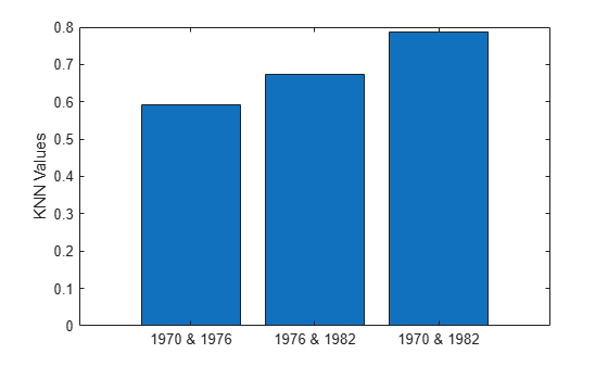
The bar graph shows that 1970 and 1976 have the smallest nearest neighbor statistic value. This result indicates that 1970 and 1976 have the most similar distribution of car measurements.

Test Two Samples for Distribution Similarity Using Nearest Neighbors

Perform a two-sample hypothesis test using a nearest neighbor statistic to determine if two iris species have the same distribution of sepal and petal dimensions. The null hypothesis of the test is that the data sets for the two iris species come from the same distribution. The alternative hypothesis is that the data sets come from different distributions.

First, perform a hypothesis test on two samples of iris data with equal numbers of each iris species. Load the fisheriris data set into a table and display the first eight rows.

fisheriris = readtable("fisheriris.csv");
head(fisheriris)

    SepalLength    SepalWidth    PetalLength    PetalWidth     Species  
    ___________    __________    ___________    __________    __________

        5.1           3.5            1.4           0.2        {'setosa'}
        4.9             3            1.4           0.2        {'setosa'}
        4.7           3.2            1.3           0.2        {'setosa'}
        4.6           3.1            1.5           0.2        {'setosa'}
          5           3.6            1.4           0.2        {'setosa'}
        5.4           3.9            1.7           0.4        {'setosa'}
        4.6           3.4            1.4           0.3        {'setosa'}
          5           3.4            1.5           0.2        {'setosa'}

Split the data set into two samples with even distribution of the species.

cv = cvpartition(fisheriris.Species,"Holdout",0.5);
sample1 = fisheriris(cv.training,:);
sample2 = fisheriris(cv.test,:);

Perform a hypothesis test at the 1% significance level using the knntest function.

[knnValue,p,h] = knntest(sample1,sample2,Alpha=0.01)

knnValue = 
0.5167

p = 
0.1364

h = 
0

The returned test decision of h = 0 indicates that knntest fails to reject the null hypothesis that the samples come from the same distribution at the 1% significance level. The value of knnValue is close to 0.5, which suggests that the samples have similar distributions.

Next, perform a hypothesis test to compare the distribution of petal and sepal data for the setosa and virginica iris species. Create separate tables containing the data for the setosa and virginica iris species.

setosa = fisheriris(string(fisheriris.Species)=="setosa",:);
virginica = fisheriris(string(fisheriris.Species)=="virginica",:);

Store the sepal and petal data for each species in a numeric matrix.

setosaData = setosa{:,1:end-1};
virginicaData = virginica{:,1:end-1};

Perform a hypothesis test at the 1% significance level using the knntest function.

[knnValue2,p2,h2] = knntest(setosaData,virginicaData,Alpha=0.01)

knnValue2 = 
1

p2 = 
2.9384e-113

h2 = 
1

The returned test decision of h = 1 indicates that knntest rejects the null hypothesis that the samples come from the same distribution at the 1% significance level. This result indicates that the setosa and virginica iris species have different distributions of sepal and petal data.

Evaluate Synthetic Tabular Data Using Nearest Neighbors

Evaluate data synthesized from an existing data set. Compare the existing and synthetic data sets to determine distribution similarity.

Load the carsmall data set, which contains measurements of cars manufactured in 1970, 1976, and 1982. Create a table containing the data and display the first eight observations.

load carsmall
carData = table(Acceleration,Cylinders,Displacement,Horsepower, ...
    Mfg,Model,Model_Year,MPG,Origin,Weight);
head(carData)

    Acceleration    Cylinders    Displacement    Horsepower         Mfg                       Model                  Model_Year    MPG    Origin     Weight
    ____________    _________    ____________    __________    _____________    _________________________________    __________    ___    _______    ______

          12            8            307            130        chevrolet        chevrolet chevelle malibu                70        18     USA         3504 
        11.5            8            350            165        buick            buick skylark 320                        70        15     USA         3693 
          11            8            318            150        plymouth         plymouth satellite                       70        18     USA         3436 
          12            8            304            150        amc              amc rebel sst                            70        16     USA         3433 
        10.5            8            302            140        ford             ford torino                              70        17     USA         3449 
          10            8            429            198        ford             ford galaxie 500                         70        15     USA         4341 
           9            8            454            220        chevrolet        chevrolet impala                         70        14     USA         4354 
         8.5            8            440            215        plymouth         plymouth fury iii                        70        14     USA         4312 

Generate 100 new observations using the synthesizeTabularData function. Specify the Cylinders and Model_Year variables as discrete numeric variables. Display the first eight observations.

rng(0,"twister")
syntheticData = synthesizeTabularData(carData,100, ...
    DiscreteNumericVariables=["Cylinders","Model_Year"]);
head(syntheticData)

    Acceleration    Cylinders    Displacement    Horsepower         Mfg                       Model                  Model_Year     MPG      Origin     Weight
    ____________    _________    ____________    __________    _____________    _________________________________    __________    ______    _______    ______

       11.215           8           309.73         137.28      dodge            dodge coronet brougham                   76          17.3    USA          4038
       10.198           8           416.68         215.51      plymouth         plymouth fury iii                        70        9.5497    USA        4507.2
       17.161           6           258.38         77.099      amc              amc pacer d/l                            76        18.325    USA        3199.8
       9.4623           8           426.19          197.3      plymouth         plymouth fury iii                        70        11.747    USA        4372.1
       13.992           4           106.63         91.396      datsun           datsun pl510                             70         30.56    Japan      1950.7
       17.965           6           266.24         78.719      oldsmobile       oldsmobile cutlass ciera (diesel)        82        36.416    USA        2832.4
       17.028           4           139.02         100.24      chevrolet        chevrolet cavalier 2-door                82        36.058    USA        2744.5
       15.343           4           118.93         100.22      toyota           toyota celica gt                         82        26.696    Japan      2600.5

Visualize the synthetic and existing data sets. Create a DriftDiagnostics object using the detectdrift function. The object's plotEmpiricalCDF and plotHistogram functions let you visualize continuous and discrete variables.

dd = detectdrift(carData,syntheticData);

Use plotEmpiricalCDF to visualize the empirical cumulative distribution function (ECDF) of the values in carData and syntheticData.

continuousVariable = "Acceleration";
plotEmpiricalCDF(dd,Variable=continuousVariable)
legend(["Existing data","Synthetic data"])

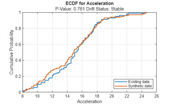
For the variable Acceleration, the ECDF of the existing data (in blue) and the ECDF of the synthetic data (in red) appear to be similar.

Use plotHistogram to visualize the distribution of values for the discrete variables in carData and syntheticData.

discreteVariable = "Cylinders";
plotHistogram(dd,Variable=discreteVariable)
legend(["Existing data","Synthetic data"])

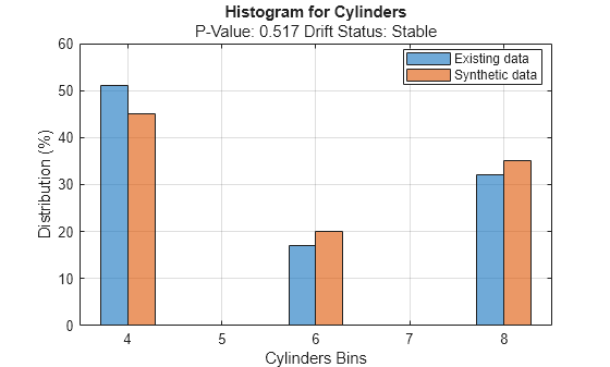
For the variable Cylinders, the distribution of data between the bins for the existing data (in blue) and the synthetic data (in red) appear similar.

Compare the synthetic and existing data sets using the knntest function. The function performs a two-sample hypothesis test for the null hypothesis that the samples come from the same distribution.

[knnstat,p,h] = knntest(carData,syntheticData)

knnstat = 
0.4933

p = 
0.6172

h = 
0

The returned value of h = 0 indicates that knntest fails to reject the null hypothesis that the samples come from different distributions at the 5% significance level. As with other hypothesis tests, this result does not guarantee that the null hypothesis is true. That is, the samples do not necessarily come from the same distribution, but both the knnstat value close to 0.5 and the high p-value indicate that the distributions of the existing and synthetic data sets are similar.

Input Arguments

X — Sample data

numeric matrix | table

Sample data, specified as a numeric matrix or a table. The rows of X correspond to observations, and the columns correspond to variables. knntest ignores observations with missing data.

• If X and Y are numeric matrices, they must have the same number of variables, but can have different numbers of observations.

• If X and Y are tables, they must have the same variable names, or the variable names of one must be a subset of the other. X and Y can have different numbers of observations.

knntest uses X as reference data to normalize continuous variables and establish a set of categories for categorical variables. When a categorical variable is in both X and Y, the variable in Y cannot contain categories that are not in X.

Data Types: single | double | table

Y — Sample data

numeric matrix | table

Sample data, specified as a numeric matrix or a table. The rows of Y correspond to observations, and the columns correspond to variables. knntest ignores observations with missing data.

• If X and Y are numeric matrices, they must have the same number of variables, but can have different numbers of observations.

• If X and Y are tables, they must have the same variable names, or the variable names of one must be a subset of the other. X and Y can have different numbers of observations.

Data Types: single | double | table

Name-Value Arguments

Specify optional pairs of arguments as Name1=Value1,...,NameN=ValueN, where Name is the argument name and Value is the corresponding value. Name-value arguments must appear after other arguments, but the order of the pairs does not matter.

Example: knntest(X,Y,NumNeighbors=15,Distance="euclidean") specifies a test that finds the 15 nearest neighbors for each observation in X and Y by using the Euclidean distance.

Alpha — Significance level

0.05 (default) | scalar value in the range (0,1)

Significance level of the hypothesis test, specified as a scalar value in the range (0,1).

Example: Alpha=0.01

Data Types: single | double

NumNeighbors — Number of nearest neighbors

10 (default) | positive integer scalar

Number of nearest neighbors to use in the computation of the statistic knnstat, specified as a positive integer scalar.

knntest uses either a Kd-tree algorithm or an exhaustive search algorithm to find the nearest neighbors. If knntest uses 10 or fewer variables in X and Y, all of which are continuous, and the Distance value is "cityblock" or "euclidean", then the function finds nearest neighbors by using a Kd-tree. Otherwise, the function uses an exhaustive search algorithm.

Example: NumNeighbors=25

Data Types: single | double

Distance — Distance metric

"seuclidean" | "hamming" | "goodall3" | "cityblock" | "correlation" | "cosine" | "euclidean" | "fasteuclidean" | "fastseuclidean"

Distance metric, specified as a character vector or string scalar.

• If all the variables are continuous (numeric), then you can specify one of these distance metrics.

  Value	Description
  "cityblock"	City block distance
  "correlation"	One minus the sample correlation between observations (treated as sequences of values)
  "cosine"	One minus the cosine of the included angle between observations (treated as vectors)
  "euclidean"	Euclidean distance
  "fasteuclidean"	Euclidean distance computed by using an alternative algorithm that saves time when the number of variables is at least 10. In some cases, this faster algorithm can reduce accuracy.
  "seuclidean"	Standardized Euclidean distance. Each coordinate difference between observations is scaled by dividing by the corresponding element of the standard deviation S = std([X Y],"omitnan").
  "fastseuclidean"	Standardized Euclidean distance computed by using an alternative algorithm that saves time when the number of variables is at least 10. In some cases, this faster algorithm can reduce accuracy.

  Note

  If you specify one of these distance metrics and the data includes categorical variables, then the software treats each categorical variable as a numeric variable for the distance computation, with each category represented by a positive integer.

• If all the variables are categorical, then you can specify the following distance metric.

  Value	Description
  "hamming"	Hamming distance, which is the percentage of coordinates that differ

  Note

  If you specify this distance metric and the data includes continuous (numeric) variables, then the software treats each continuous variable as a categorical variable for the distance computation.

• If the variables are a mix of continuous (numeric) and categorical variables, then you can specify the following distance metric.

  Value	Description
  "goodall3"	Modified Goodall distance

The default value is "seuclidean" if all the variables are continuous, "hamming" if all the variables are categorical, and "goodall3" if the variables are a mix of continuous and categorical variables. For more information on the various distance metrics, see Distance Metrics.

Example: Distance="euclidean"

Data Types: char | string

VariableNames — Variables to include in computation

character vector | string array | cell array of character vectors

Variables to include in the computation, specified as a character vector, string array, or cell array of character vectors. Because matrices do not have named variables, this argument applies only when X and Y are tables.

• VariableNames must be a subset of the variables shared by X and Y.

• By default, VariableNames contains all the variables shared by X and Y.

Example: VariableNames=["Name","Age","Score"]

Data Types: char | string | cell

CategoricalVariables — Variables to treat as categorical

"all" | vector of numeric indices | logical vector | string array | cell array of character vectors

Variables to treat as categorical, specified as one of the values in this table.

Value	Description
"all"	All variables contain categorical values.
Vector of numeric indices	Each vector element corresponds to the index of a variable, indicating that the variable contains categorical values.
Logical vector	A logical vector the same length as VariableNames. A value of true indicates that the corresponding variable contains categorical values.
String array or cell array of character vectors	An array containing the names of variables with categorical values. The array elements must be names found in VariableNames.

If X and Y are numeric matrices, then CategoricalVariables cannot be a string array or cell array of character vectors. By default, knntest assumes all variables in numeric matrices are continuous, and treats table columns of character arrays or string scalars as categorical variables.

Example: CategoricalVariables="all"

Data Types: single | double | logical | char | string | cell

Output Arguments

knnstat — Nearest neighbor statistic

scalar value in the range [0,1]

Nearest neighbor statistic, returned as a scalar value in the range [0,1]. If X and Y are well separated, then the knnstat value is close to 1. If X and Y are similar data sets with the same number of observations, then the knnstat value tends to be close to 0.5. For more information, see Nearest Neighbor Statistic.

p — p-value

scalar value in the range [0,1]

p-value of the test, returned as a scalar value in the range [0,1]. p is the probability of observing a test statistic that is as extreme as, or more extreme than, the observed value under the null hypothesis. A small value of p indicates that the null hypothesis might not be valid.

h — Hypothesis test result

1 | 0

Hypothesis test result, returned as 1 or 0.

• A value of 1 indicates the rejection of the null hypothesis at the Alpha significance level.

• A value of 0 indicates a failure to reject the null hypothesis at the Alpha significance level.

More About

Distance Metrics

A distance metric is a function that defines a distance between two observations. knntest supports various distance metrics for continuous (numeric) variables, categorical variables, and a mix of continuous and categorical variables. To specify the distance metric to use for computing the nearest neighbor statistic, set the Distance name-value argument of knntest.

Given an mx-by-n data matrix X, which is treated as mx (1-by-n) row vectors x₁, x₂, ..., x_mx, and an my-by-n data matrix Y, which is treated as my (1-by-n) row vectors y₁, y₂, ...,y_my, the various distances between the vector x_s and y_t are defined as follows:

• City block distance

  $$d_{st}={\displaystyle \sum _{j=1}^n\left|x_{sj}-y_{tj}\right|}.$$

  The city block distance is a special case of the Minkowski distance, where p = 1.

• Correlation distance

  $$d_{st}=1-\frac{\left(x_s-{\overline{x}}_s\right){\left(y_t-{\overline{y}}_t\right)}^{\prime }}{\sqrt{\left(x_s-{\overline{x}}_s\right){\left(x_s-{\overline{x}}_s\right)}^{\prime }}\sqrt{\left(y_t-{\overline{y}}_t\right){\left(y_t-{\overline{y}}_t\right)}^{\prime }}},$$

  where

  $${\overline{x}}_s=\frac{1}{n}{\displaystyle \sum _j{x}_{sj}}$$

  and

  $${\overline{y}}_t=\frac{1}{n}{\displaystyle \sum _j{y}_{tj}}.$$

• Cosine distance

  $$d_{st}=\left(1-\frac{x_s{y^{\prime }}_t}{\sqrt{\left(x_s{x^{\prime }}_s\right)\left(y_t{y^{\prime }}_t\right)}}\right).$$

• Euclidean distance

  $$d_{st}^2=(x_s-y_t)(x_s-y_t{)}^{\prime }.$$

  The Euclidean distance is a special case of the Minkowski distance, where p = 2.

• Fast Euclidean distance

  The fast Euclidean distance is the same as the Euclidean distance, but is computed using an alternative algorithm that saves time when the number of variables is at least 10. In some cases, this faster algorithm can reduce accuracy. For more information, see Fast Euclidean Distance Algorithm.

• Hamming distance

  $$d_{st}=(\#(x_{sj}\ne y_{tj})/n).$$

  The Hamming distance is the percentage of coordinates that differ.

• Modified Goodall distance

  The modified Goodall distance is a variant of the Goodall distance, which assigns a small distance if the matching values are infrequent regardless of the frequencies of the other values. For mismatches, the distance contribution of the variable is 1/(number of variables).

• Standardized Euclidean distance

  $$d_{st}^2=(x_s-y_t)V^{-1}(x_s-y_t{)}^{\prime },$$

  where V is the n-by-n diagonal matrix whose jth diagonal element is (S(j))², where S is a vector of scaling factors for each dimension.

• Fast standardized Euclidean distance

  The fast standardized Euclidean distance is the same as the standardized Euclidean distance, but is computed using an alternative algorithm that saves time when the number of variables is at least 10. In some cases, this faster algorithm can reduce accuracy. For more information, see Fast Euclidean Distance Algorithm.

Tips

• Avoid specifying small values for NumNeighbors (such as NumNeighbors=1 or NumNeighbors=2). knntest assumes that the number of nearest neighbors, the number of observations in X and Y, and the number of variables in X and Y are sufficiently large. For more information, see [1].

Algorithms

Nearest Neighbor Statistic

The nearest neighbor statistic knnstat indicates how well separated the X and Y data sets are, based on whether the observations' nearest neighbors tend to be in the same set as the observations.

Suppose m is the total number of observations in X and Y combined. Define an m-by-NumNeighbors matrix I, where each row corresponds to an observation in X or Y, and each column corresponds to a nearest neighbor. Let I(i,j) = 1 if observation i and its nearest neighbor j are in the same data set, and I(i,j) = 0 otherwise. The statistic knnstat is equal to mean(I,"all").

If X and Y are well separated, then the knnstat value is close to 1. If X and Y are similar data sets with the same number of observations, then the knnstat value tends to be close to 0.5. For more information, see [1].

p-Value Computation and Hypothesis Test

To determine p and h, the knntest function uses a right-tailed hypothesis test that assumes the test statistic (knnstat – μ)/σ has a standard normal distribution.

• μ is defined as:

  $$\mu =\frac{m_x(m_x-1)+m_y(m_y-1)}{m(m-1)}$$

  • m_x is the number of observations in X.

  • m_y is the number of observations in Y.

  • m is the total number of observations in X and Y.

• σ² is defined as:

  $${\sigma }^2=\frac{1}{m\cdot k}\left(\frac{m_x\cdot m_y}{m^2}+4{\left(\frac{m_x\cdot m_y}{m^2}\right)}^2\right)$$

  • k is the number of nearest neighbors specified by the NumNeighbors name-value argument.

The normal distribution assumption is based on the limiting behavior of the test statistic as k, m, and the number of variables in X and Y increase. For more information, see [1].

References

[1] Williams, M. “How Good Are Your Fits? Unbinned Multivariate Goodness-of-Fit Tests in High Energy Physics.” Journal of Instrumentation 5, no. 09 (September 9, 2010): P09004. https://doi.org/10.1088/1748-0221/5/09/P09004.

Version History

Introduced in R2025a