Model Reference Adaptive Control

The Model Reference Adaptive Control block computes control actions to make an uncertain controlled system track the behavior of a given reference plant model. Using this block, you can implement the following model reference adaptive control (MRAC) algorithms.

• Direct MRAC — Estimate the feedback and feedforward controller gains based on the real-time tracking error between the states of the reference plant model and the controlled system.

• Indirect MRAC — Estimate the parameters of the controlled system based on the tracking error between the states of the reference plant model and the estimated system. Then, derive the feedback and feedforward controller gains based on the parameters of the estimated system and the reference model.

Both direct and indirect MRAC also estimate a model of the external disturbances and uncertainty in the system being controlled. The controller then uses this model to compensate for the disturbances and uncertainty when computing control actions.

In both cases, the controller updates the estimated parameters and disturbance model in real-time based on the tracking error.

Reference Model

For both direct and indirect MRAC, the following reference plant model is the ideal system that characterizes the desired behavior that you want to achieve in practice.

$${\dot{x}}_m\left(t\right)=A_m{x}_m\left(t\right)+B_{m}r\left(t\right)$$

Here:

• r(t) is the external reference signal.

• x_m(t) is the state of the reference plant model. Since r(t) is known, you can simulate the reference model to get x_m(t).

• A_m is a constant state matrix. For a stable reference model, A_m must be a Hurwitz matrix for which every eigenvalue must have a strictly negative real part.

• B_m is a control effective matrix.

Disturbance and Uncertainty Model

The Model Reference Adaptive Control block maintains an internal model u_ad of the disturbance and model uncertainty in the controlled system.

$$u_{ad}=w^T\varphi \left(x\right)$$

Here, ϕ(x) is a vector of model features. w is an adaptive control weight vector that the controller updates in real time based on the tracking error.

To define ϕ(x), you can use one of the following feature definitions.

• State vector of the controlled plant — This approach can under-represent the uncertainty in the system. Using the states as features can be a useful starting point when you do not know the complexity of the disturbance and model uncertainty.

• Gaussian radial basis functions — Use this option when the disturbance and model uncertainty are nonlinear and the structure of the disturbance model is unknown. Radial basis functions require some prior knowledge of the operation domain of the model, which can be difficult for some cases.

• Single hidden layer neural network — Use this option when the disturbance and model uncertainty are nonlinear and the structure of the disturbance model is unknown and you do not have prior knowledge of the operating domain. The neural network is a universal function approximator that can approximate any continuous function.

• External source provided to the controller block — Use this option to define your own custom feature vector. You can use this option when you know the structure of the disturbance and uncertainty model. For example, you can use a custom feature vector to identify specific unknown plant parameters.

Direct MRAC

A direct MRAC controller has the following control structure.

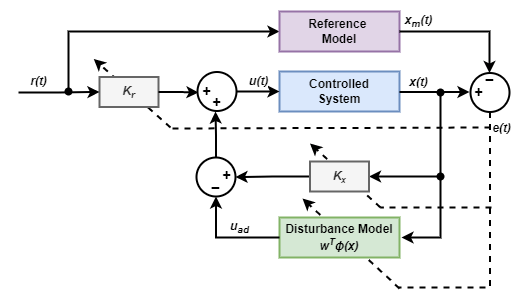
The controller computes the control input u(t) as follows.

$$\begin{array}{l}u\left(t\right)=k_{x}x\left(t\right)+k_{r}r\left(t\right)-u_{ad}\\ u_{ad}=w^T\varphi \left(x\right)\end{array}$$

Here:

• x(t) is the state of the controlled system.

• r(t) is the external reference signal.

• k_x and k_r are the feedback and feedforward controller gains, respectively.

• u_ad is the adaptive control component derived from the disturbance model.

  ϕ(x) contains the disturbance model features.

• w is an adaptive disturbance model weight vector.

• V is the hidden layer weight vector.

For a single hidden layer neural network, u_ad is:

$$u_{ad}=w^T\sigma \left(V^{T}x\right)$$

Here:

• V is the hidden layer weight vector.

• σ is a sigmoid activation function.

The controller computes the error e(t) between the states of the controlled system and the states of the reference model. It then uses that error to adapt the values of k_x, k_r, and w in real time.

Nominal Model

The controlled system, which typically exhibits modeling uncertainty and external disturbances, has the following nominal state equation. The controller uses this expected nominal plant behavior when updating the controller parameters.

$$\dot{x}\left(t\right)=Ax\left(t\right)+B\left(u\left(t\right)+f\left(x\right)\right)$$

Here:

• x(t) is the state of the system you want to control.

• u(t) is the control input.

• A is a constant state-transition matrix.

• B is a constant control effective matrix.

• f(x) is the matched uncertainty in the system.

Parameter Updates

A direct MRAC controller uses the following equations to update the controller gains and disturbance model weights for state vector, radial basis function, and external source feature definitions [1] [2].

$$\begin{array}{l}{\dot{k}}_x={\Gamma }_{x}x\left(t\right)e^T\left(t\right)PB\\ {\dot{k}}_r={\Gamma }_{r}r\left(t\right)e^T\left(t\right)PB\\ \dot{w}={\Gamma }_w\varphi \left(x\right)e^T\left(t\right)PB\end{array}$$

A single hidden layer disturbance model update equations use the same controller gain updates along with the following update equations.

$$\begin{array}{l}\dot{w}=-\left(\sigma \left(V^{T}x\right)-{\sigma }^{\prime }\left(V^{T}x\right)V^{T}x\right)e^T\left(t\right)PB{\Gamma }_w\\ \dot{V}=-{\Gamma }_{V}x{e}^T\left(t\right)PB{w}^T\sigma \left(V^{T}x\right)\end{array}$$

Here, P is the solution to the following Lyapunov function based on the reference model state matrix and B is the control effective matrix from the nominal plant model.

$$A_m^{T}P+P{A}_m+Q=0$$

Here, Q is a positive definite matrix of size N-by-N, where N is size of state vector x(t)

Indirect MRAC

An indirect MRAC controller has the following control structure. The reference model is

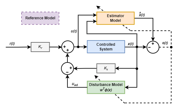
The controller computes the control input u(t) as follows.

$$\begin{array}{l}u\left(t\right)=k_{x}x\left(t\right)+k_{r}r\left(t\right)-u_{ad}\\ u_{ad}=w^T\varphi \left(x\right)\end{array}$$

Here:

• $$\widehat{x}$$(t) is the estimated state of the controlled system produced by an estimator model.

• r(t) is the external reference signal.

• k_x and k_r are the feedback and feedforward controller gains, respectively.

• u_ad is the adaptive control component derived from the disturbance model.

  ϕ(x) contains the disturbance model features.

• w is an adaptive disturbance model weight vector.

The controller computes the error e(t) between the actual and estimated system states. It then uses that error to adapt the values of w in real time. The controller also uses e(t) to update the parameters of the estimator model in real time. The values of gains k_x and k_r are derived from the parameters of the estimator model and reference model.

Estimator Model and Controller Gains

The indirect MRAC controller contains the following estimator model of the controlled system.

$$\dot{\widehat{x}}\left(t\right)=\widehat{A}x\left(t\right)+\widehat{B}u\left(t\right)$$

Here:

• $$\widehat{x}$$(t) is the estimated system state.

• u(t) is the control input.

• $$\widehat{A}$$ is the state-transition matrix of the estimator.

• $$\widehat{B}$$ is the control effective matrix of the estimator.

During operation the controller updates $$\widehat{A}$$ and $$\widehat{B}$$ based on the estimation error e(t).

Rather than estimate the controller gains directly, an indirect MRAC controller derives the feedback gain k_x and feedforward gain k_r from the parameters of the reference and estimator models using a dynamic inversion-based approach as follows.

$$\begin{array}{l}{k}_r=\frac{B_m}{\widehat{B}}\\ k_x=\frac{1}{\widehat{B}}\left(A_m-\widehat{A}\right)\end{array}$$

Here, $$\frac{1}{\widehat{B}}$$ is the Moore-Penrose pseudoinverse of the matrix $$\widehat{B}$$.

Parameter Updates

An indirect MRAC controller uses the following equations to update the estimator model parameters and disturbance model weights for state vector, radial basis function, and external source feature definitions [1] [2].

$$\begin{array}{l}\dot{\widehat{A}}={\Gamma }_{a}x\left(t\right)e^T\left(t\right)P\\ \dot{\widehat{B}}={\Gamma }_{b}u\left(t\right)e^T\left(t\right)P\\ \dot{w}={\Gamma }_w\varphi \left(x\right)e^T\left(t\right)PB\end{array}$$

A single hidden layer disturbance model update equations use the same estimator model parameter updates along with the following update equations.

$$\begin{array}{l}\dot{w}=-\left(\sigma \left(V^{T}x\right)-{\sigma }^{\prime }\left(V^{T}x\right)V^{T}x\right)e^T\left(t\right)PB{\Gamma }_w\\ \dot{V}=-{\Gamma }_{V}x{e}^T\left(t\right)PB{w}^T\sigma \left(V^{T}x\right)\end{array}$$

Here, P is the solution to the following Lyapunov function.

$$k_{\tau }^{T}P+P{k}_{\tau }+Q=0$$

k_τ is the estimator feedback gain. By default, this value corresponds to the reference model state-transition matrix A_m. However, you can specify a different estimator feedback gain value.

Learning Modification

For both direct and indirect MRAC, to add robustness at higher learning rates, you can modify the parameter updates to include an optional momentum term. You can choose one of two possible learning modification methods: sigma modification and e-modification.

For sigma modification, the momentum term for each parameter update is the product of the momentum weight parameter σ and the current parameter value. For example, the following update equations for a direct MRAC controller include a sigma modification term.

$$\begin{array}{l}{\dot{k}}_x={\Gamma }_{x}x\left(t\right)e^T\left(t\right)PB+\sigma k_x\\ {\dot{k}}_r={\Gamma }_{r}r\left(t\right)e^T\left(t\right)PB+\sigma k_x\\ {\dot{w}}_x={\Gamma }_w\varphi \left(t\right)e^T\left(t\right)PB+\sigma w\end{array}$$

For e-modification, the controller scales the sigma-modification momentum term by the norm of the error vector. For example, the following update equations for an indirect MRAC controller include an e-modification term.

$$\begin{array}{l}\dot{\widehat{A}}={\Gamma }_{a}x\left(t\right)e^T\left(t\right)P+\sigma \left|e\left(t\right)\right|\widehat{A}\\ \dot{\widehat{B}}={\Gamma }_{b}u\left(t\right)e^T\left(t\right)P+\sigma \left|e\left(t\right)\right|\widehat{B}\\ {\dot{w}}_x={\Gamma }_w\varphi \left(t\right)e^T\left(t\right)PB+\sigma \left|e\left(t\right)\right|w\end{array}$$

To adjust the amount of the learning modification for either method, change the value of the momentum weight parameter σ.

More About Model Reference Adaptive Control

For more information on model reference adaptive control, play the video. This video is part of the Learning-Based Control video series.

References

[1] Ioannou, Petros A., and Jing Sun. Robust Adaptive Control, Courier Corporation, 2012.

[2] Narendra, Kumpati S, and Anuradha M Annaswamy. Stable Adaptive Systems. Courier Corporation, 2012.

[3] Narendra, Kumpati S., and Anuradha M. Annaswamy. “Robust Adaptive Control.” In 1984 American Control Conference, 333–35. San Diego, CA, USA: IEEE, 1984. https://doi.org/10.23919/ACC.1984.4788398.