Load Data to Model Variable-Step Input from Model Hierarchy

A model hierarchy can include discrete and continuous components that operate with different dynamics. You might simulate a model hierarchy that contains both discrete and continuous components using a variable-step solver.

As you develop each component, you can simulate the referenced model that implements the component as a top model. Instead of the input data coming from the model hierarchy, the Inport block loads external input data you specify using the Input model configuration parameter.

This example shows how you can use the Output times model configuration parameter to ensure such a simulation captures dynamics of continuous input signals logged from a variable-step simulation. For more information, see Control How Models Load Input Data.

Open Top Model

Open the model ContinuousPlant. The model contains a Transfer Fcn block that models a continuous plant. A Step block provides the input for the continuous plant. The plant output signal is connected to an output port and a referenced model that processes the signal using a discrete algorithm. The algorithm counts the number of oscillations that reach a value of 1.5 or higher. The top model uses a variable-step solver to capture the continuous dynamics of the plant.

mdl = "ContinuousPlant";
open_system(mdl)

Simulate Top Model

Suppose you want to test and refine the model CountOscillations in isolation. You can use data logged from a simulation of the top model as input data when you simulate the referenced model as a top model.

Simulate the top model. On the Simulink® Toolstrip, on the Simulation tab, click Run. Alternatively, use the sim function.

out = sim(mdl);

Get the logged data for the two outputs Step Response and Oscillation Count.

yout = out.yout;
stepResp = getElement(yout,"Step Response");
oscCount = getElement(yout,"Oscillation Count");

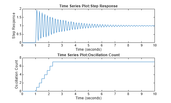
Plot the plant step response. The plot shows that the step response is underdamped and the algorithm counts 7 oscillations that go above a value of 1.5.

figure(1)
subplot(2,1,1)
plot(stepResp.Values)
subplot(2,1,2)
plot(oscCount.Values)

Simulate Referenced Model as Top Model

Open the model CountOscillations as a top model.

mdl2 = "CountOscillations";
open_system(mdl2)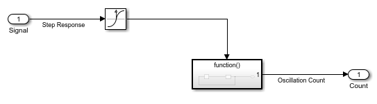

Configure the model to load the data in the variable stepResp as simulation input.

1. In the Simulink Toolstrip, on the Modeling tab, click Model Settings.

2. Select the Data Import/Export pane.

3. Select Input.

4. In the Input field, enter stepResp.

5. Click OK.

Alternatively, you can configure the simulation to load the external input data programmatically, using a Simulink.SimulationInput object.

Create a Simulink.SimulationInput object for the referenced model. Then, use the setExternalInput function to specify the external input for the simulation as the variable stepResp.

simIn = Simulink.SimulationInput(mdl2);
simIn = setExternalInput(simIn,"stepResp");

To see how the model loads the input data, mark the input signal for logging. Select the signal Step Response. Then, in the Simulation tab, click Log Signals.

Alternatively, you can mark the signal for logging using the Simulink.sdi.markSignalsForStreaming function.

blkPth = strcat(mdl2,"/Signal");
Simulink.sdi.markSignalForStreaming(blkPth,1,"on")

Simulate the model.

out2 = sim(simIn);

Get the data for the logged input signal and the oscillation count.

logsout = out2.logsout;
stepRespInput = getElement(logsout,"Step Response");

yout2 = out2.yout;
oscCount2 = getElement(yout2,"Oscillation Count");

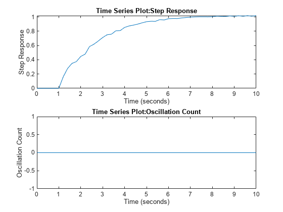
Plot the input signal and the oscillation count. The response appears no longer underdamped, and the algorithm counts zero oscillations due to the way the simulation loaded the step response data.

figure(2)
subplot(2,1,1)
plot(stepRespInput.Values)
subplot(2,1,2)
plot(oscCount2.Values)

When you simulate the referenced model as a top model, the solver is aware of the step response dynamics only after the Inport block loads the input data into the model. Because the signal had continuous sample time in a variable-step simulation, the samples are not evenly spaced. To load the data in a way that accurately reflects the step response, the Inport block needs to load more input values from the step response data.

Specify Additional Output Times for Simulation

You can use the Output times model configuration parameter to force the variable-step solver to take time steps at specified values in addition to those the solver determines. You can use the time values in the logged data from the first simulation to specify the value of the Output times parameter.

For this example, because the oscillations in the step response continue throughout the simulation, specify the value of the Output times parameter as the entire time vector for the input data. Get the vector of time values.

outTimes = stepResp.Values.Time;

Specify the Output times parameter value as the variable outTimes.

1. In the Simulink Toolstrip, on the Modeling tab, click Model Settings.

2. Select the Data Import/Export tab.

3. Expand Additional parameters.

4. Set Output options to Produce additional output.

5. In the Output times field, type outTimes.

6. Click OK.

Alternatively, you can configure the parameter values for the simulation using the SimulationInput object.

simIn = setModelParameter(simIn,...
    "OutputOption","AdditionalOutputTimes",...
    "OutputTimes","outTimes");

Simulate the model again.

out3 = sim(simIn);

Get the data for the logged input signal and the oscillation count.

logsout2 = out3.logsout;
stepRespInput2 = getElement(logsout2,"Step Response");

yout3 = out3.yout;
oscCount3 = getElement(yout3,"Oscillation Count");

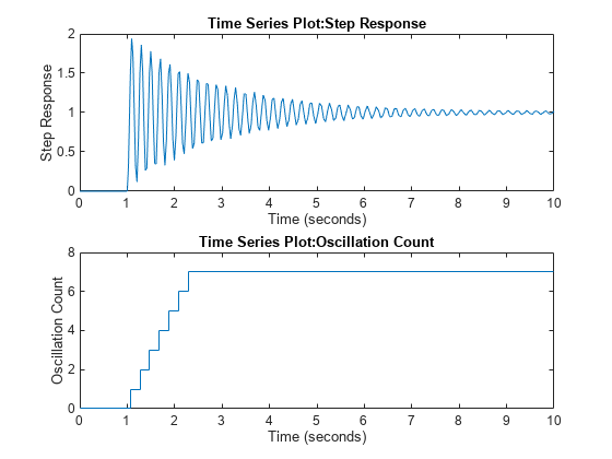
Plot the logged input signal and the oscillation count. Now, the plots look the same as those from the first simulation of the entire model hierarchy.

figure(3)
subplot(2,1,1)
plot(stepRespInput2.Values)
subplot(2,1,2)
plot(oscCount3.Values)

Depending on the requirements for your system, you can specify the value for the Output times parameter using the time vector for the entire input signal or using one or more relevant portions of the input signal time data.

To extract portions of a timeseries object, you can create a tsdata.event object that describes a point of interest within the timeseries and then use a function such as gettsbeforeevent or gettsafterevent to extract the desired portion of the timeseries object. Then, you can use the time vector for one or more of these timeseries objects to specify the value for the Output times parameter.