Control How Models Load Input Data
When you load external input data, the time values you specify in external input data do not determine how the model loads the data during simulation. The solver determines which time steps to take in simulation. The sample time for the block that loads the data determines when the block executes and provides a new signal value. The solver can consider the dynamics of the input data only after the loading block loads each value into the model.
You can use model parameters, block parameters, and different input data formats to ensure that your model loads your input data as you expect.
Configure Input Data Interpolation
When you load external input data, the time steps the solver chooses typically do not match the time steps you specify for external inputs. When the simulation takes a time step that does not match a time value provided in the external input data, the software uses the time and data values in the external input data to interpolate the signal value.
You can configure how a loading block interpolates the data it loads using block parameters. The table summarizes how to configure available interpolation options for each loading block.
| Loading Block | Interpolation Options |
|---|---|
Linear interpolation — Select Interpolate data. Zero-order hold — Clear Interpolate data. | |
Configure the interpolation for each input signal by selecting the signal from the Active Signal list. Linear interpolation — Select Interpolate data. Zero-order hold — Clear Interpolate data. | |
| In Bus Element | Always linearly interpolates input data. |
Linear interpolation — Set Data interpolation within time
range to Zero-order-hold — Set Data
interpolation within time range to | |
| Playback | Configure the interpolation for the input data using the Interp Method property for the signal or message. Linear
interpolation — Set Interp Method to
Zero-order hold — Set
Interp Method to
No interpolation — Set
Interp Method to |
Capture Dynamics of Input Data
The solver considers the dynamics of external input data, such as discontinuities and transient variations, only after a loading block loads the data into the simulation. For blocks with continuous sample time, the solver also determines when the block executes. When the external input data changes faster than the system dynamics, the solver can miss dynamics in the input data that can affect the simulation. If the simulation takes too large of a step for your input data, you can take one of these actions to ensure the signal produced in the model reflects your input data:
| Action | Details and Considerations |
|---|---|
| Specify a sample time for the loading block | The sample time for a block specifies when the block executes in
simulation. You can specify the sample time for a block as something other than
inherited ( This strategy might introduce a new sample time into your model or cause extraneous time steps when the input signal changes gradually. |
| Specify required time steps for variable-step simulations using the Output times model configuration parameter | The Output times parameter for a model specifies times of interest for variable-step simulations. When you specify a value for the Output times parameter, the solver takes a major time step for each time value. You can specify the value for the Output times parameter using all or part of the time vector for your input data. This parameter does not affect time steps for simulations that use a fixed-step solver. |
| Configure a root-level input port to use input events | When you configure a root-level input port to use input events, the
external input data drives the execution of the block. The Only Inport blocks and In Bus Element blocks support input events. When you use input events, you must specify a partition of your model to execute each time the input event occurs. |
Load Data as Continuous Signal
A continuous signal has a value at any time point. When the loading block has constant (0) sample time, the block executes and provides an output value for the continuous signal for every time step in the simulation. To load input data as a continuous signal, use a data format that includes time values and use linear interpolation.
Open and Examine Model
Open the model LoadInputData. The model uses an Inport block to load external input data from the base workspace.
mdl = "LoadInputData";
open_system(mdl);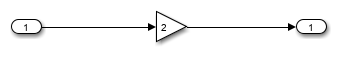
The Input parameter for the model is configured to load data from the variable simIn.
get_param(mdl,"LoadExternalInput")ans = 'on'
get_param(mdl,"ExternalInput")ans = 'simIn'
Create and Format Input Data
Create data for a sine wave in the base workspace. You can load data from the workspace using several formats, most of which fundamentally consist of signal values paired with time values. For this example, use the timetable format.
First, create a column vector of time values.
sampleTime = 0.1;
numSteps = 101;
time = sampleTime*(0:numSteps-1);
time = time';
To create a timetable, the time data must be a duration vector. Use the seconds function to create a duration vector with units of seconds.
secs = seconds(time);
Use the sin function to create the signal values for each value in the time vector.
data = sin(2*pi/3*time);
Create the timetable object.
simIn = timetable(secs,data);
Configure Inport Block to Produce Continuous Signal
Configure the Inport block to have continuous sample time and to linearly interpolate the input data during simulation.
Select the Inport block.
Open the Property Inspector by clicking the Property Inspector tab on the right of the model or by pressing Ctrl+Shift+I.
Expand the Execution section.
Set the Sample time to
0to use continuous sample time.Select Interpolate data.
Alternatively, use the set_param function to set the block parameters.
set_param(strcat(mdl,"/Inport"),"SampleTime","0",...
    "Interpolate","on")
Simulate Model
Simulate the model by clicking Run or by using the sim function.
contOut = sim(mdl);
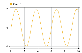
The Dashboard Scope block shows the output signal as a smooth, continuous sine wave.
Load Data as Discrete Signal
The values for a discrete signal change only at specific times, typically represented as an evenly spaced vector of sample times. Between each sample of the signal, the signal value remains the same. To load input data as a discrete signal, choose an input data format, use zero-order-hold interpolation, and specify a sample time for the loading block.
Open and Examine Model
Open the model LoadInputData. The model uses an Inport block to load external input data from the base workspace.
mdl = "LoadInputData";
open_system(mdl)
The Input parameter is configured to load data from the variable simIn.
get_param(mdl,"LoadExternalInput")ans = 'on'
get_param(mdl,"ExternalInput")ans = 'simIn'
Create and Format Input Data
Create input data for a sine wave in the base workspace. To start, create an evenly spaced time vector to pass to the sin function to generate the data values.
When you create data to load as a discrete signal, use the expression in this example. Other techniques for creating an evenly spaced time vector, such as the linspace function or using the colon operator with a specified increment (a:b:c), can introduce floating-precision rounding errors that can lead to unexpected simulation results.
sampleTime = 0.1;
numSteps = 101;
time = sampleTime*(0:numSteps-1);
time = time';
Create the signal values by using the sin function to create a value for each element in the time vector.
data = sin(2*pi/3*time);
Format the workspace data to load into the simulation. When you load input data for a discrete signal, you can avoid the effect of floating-precision rounding errors in data you provide by using the structure without time format.
When you use the structure without time format, you do not specify time data along with the signal values. Instead, the simulation associates time values with the signal values using the sample time you specify for the block. During simulation, the block loads the input values sequentially at the specified rate.
The structure format has two fields:
time: A common time vector for all signals in the structuresignals: An array of structures that contain the data and dimensions information for each signal
Create the structure simIn to load the sine wave data into the model using the structure without time format.
simIn.signals.values = data;
simIn.signals.dimension = 1;
simIn.time = [];
Configure Block to Produce Discrete Signal
Configure the block to use a sample time of 0.1 and use zero-order-hold interpolation.
Select the Inport block.
Open the Property Inspector by clicking the Property Inspector tab on the right of the model or by pressing Ctrl+Shift+I.
Expand the Execution section.
Set the Sample time to
0.1.Clear Interpolate data.
Alternatively, use the set_param function to configure the block.
set_param(strcat(mdl,"/Inport"),"SampleTime","0.1",...
    "Interpolate","off")
Simulate Model
Simulate the model.
out = sim(mdl);
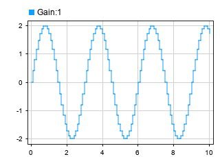
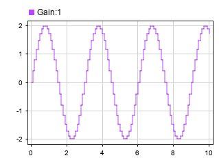
The Dashboard Scope block displays the sine wave signal. The zero-order hold creates a stair step effect between each sample value.
Use Format with Time Data
When you create the evenly spaced time vector yourself, using the expression in this example, you can also load input data using formats that include time values without floating-precision rounding issues. For example, create a timetable using the time and signal values for the sine wave.
secs = seconds(time);
simIn = timetable(secs,data);
Simulate the model again.
out2 = sim(mdl);
The results on the Dashboard Scope look the same as the previous simulation.
The values in the time vector are the same for the simulation that used the structure without time format and the simulation that used the timetable format with a time vector created using the expression in this example.
isequal(out.yout{1}.Values.Time,out2.yout{1}.Values.Time)ans = logical
1
Load Message Data into Model Using Playback Block
When you have data in a file, the workspace, or the Simulation Data Inspector, you can use the Playback block to load the data into your model as messages. To load input data as messages, specify the interpolation method of your signal as none. In Simulink®, a message is a modeling artifact that combines events with related data. For more information about messages, see Simulink Messages Overview.
Open and Examine Model
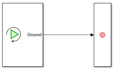
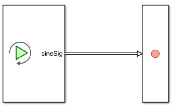
Open the model PlaybackRecord. The model contains an empty Playback block connected to a Record block. Once you add data, the Playback block loads external data into the model during simulation. The Record block logs output data from the Playback block.
Add Data to Playback Block
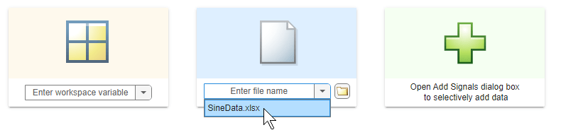
The Microsoft® Excel® file SineData contains discrete data for a sine wave signal named sineSig. To add data from the SineData file to the Playback block, double-click the block. Then, from the file selection drop-down list, select the SineData file.
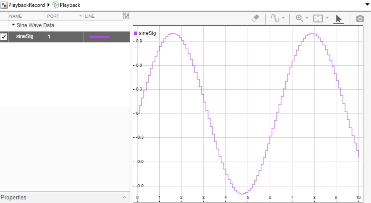
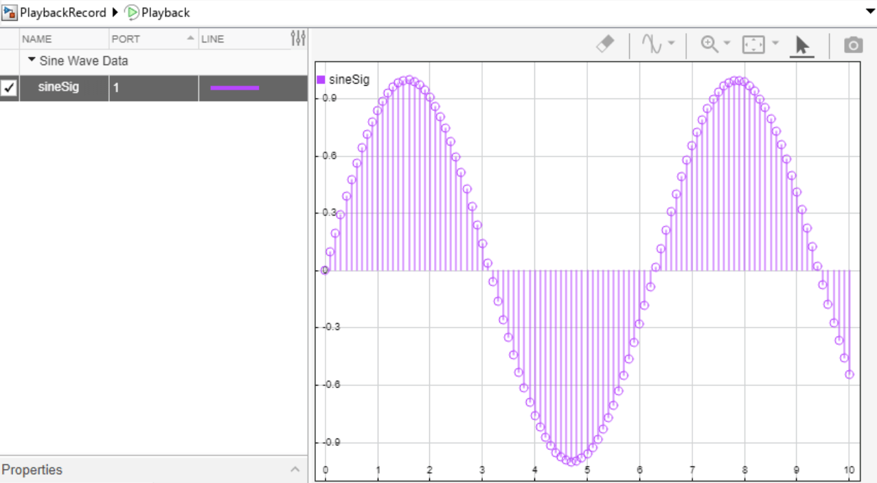
The Playback block plots the added signal sineSig in a sparkline plot so that you can visually inspect the data before loading signals into the model. The plot displays the signal using the default ZOH interpolation because the data in the file did not specify the interpolation for the signal. The interpolation property for the signal in the Playback block specifies both how the Playback block displays the signal in the plot and how the Playback block loads the data into the model.
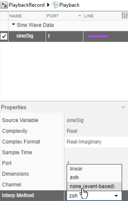
Configure Block to Produce Messages
To have the Playback block load signal values as message payloads, set the interpolation method to none. Select the sineSig signal. Then, in the Properties pane, set Interp Method to none (event-based).
Alternatively, you can include metadata in the Excel spreadsheet to specify the interpolation method as none. For more information, see Microsoft Excel Import, Export, and Logging Format.
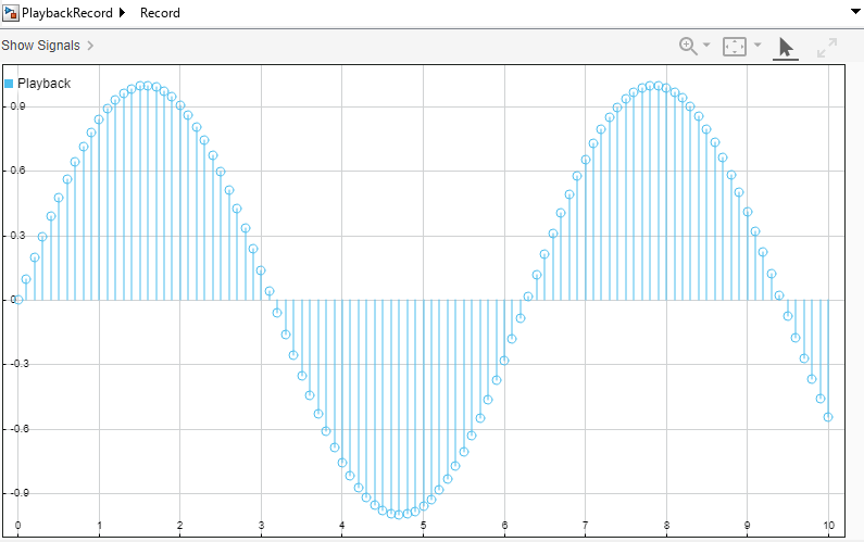
When the Playback block loads a signal that is not interpolated, the block produces messages. The Playback block displays a stem plot where the value of each stem is the payload value of the produced message at that simulation time.
Load Data into Model and Visualize Output
Simulate the model. The Playback block loads data into the model when you run a simulation. During simulation, the Record block logs the output from the Playback block. Observe that the line style of the connection between the Playback block and the Record block is now a message line.
Double-click the Record block to visualize the logged data.