plot
R2026bDescription
plot( plots the entire hybrid pulse
power characterization (HPPC) test voltage over time, showing the identified charge and
discharge pulse indices.myHppcTest)
plot(
plots the HPPC test voltage and specifies options using one or more name-value
arguments.myHppcTest,Name=Value)
chart = plot(___)HPPCChart object.
Examples
This example shows how to plot the entire hybrid pulse power characterization (HPPC) test voltage over time.
Open the DownloadBatteryData example and load the required HPPC
data obtained for a BAK 2.9 Ah battery cell at 25 °C. This data consists of a table with
three columns. The columns of the table refer to time, voltage, and current values,
respectively.
openExample("simscapebattery/DownloadBatteryDataExample")
load("testDataBAKcells/hppcDataBAKcell25degC.mat")
Store the HPPC data inside an HPPCTest object by using the hppcTest function. You can use this object
to view the data, add or edit breakpoints, add or remove pulses, and include additional
information such as state of charge and capacity. The HPPC data is a table, so you must
also specify each column name by using the TimeVariable,
VoltageVariable, and CurrentVariable arguments.
These names must match the names of the columns in the hppcData
table.
hppcExp = hppcTest(hppcData,...
    TimeVariable="time (s)",...
    VoltageVariable="voltage (V)",...
    CurrentVariable="current (A)");
Analyze the TestSummary property of the
hppcExp object. This property contains a summary of the HPPC test
that shows all the identified pulses and related data, returned as a table.
hppcExp.TestSummary
ans =

  18×13 table

    PulseID    Directionality      SOC          HPPCData         PulseDuration    PseudoOCV_V    MaximumVoltage    MinimumVoltage    Current_A    C_rate    PulseStartIndex    PulseEndIndex    Temperature_degC
    _______    ______________    _______    _________________    _____________    ___________    ______________    ______________    _________    ______    _______________    _____________    ________________

       1        "Discharge"            1    {701×6 timetable}         30            4.1745           4.1745            3.7846         -6.1869     1.8976           354              1055               25
       2        "Discharge"      0.90376    {701×6 timetable}         30            4.0837           4.0837            3.7479          -6.187     1.8977          2702              3403               25
       3        "Discharge"      0.80754    {702×6 timetable}         30            4.0132           4.0132            3.6652         -6.1867     1.8975          5049              5751               25
       4        "Discharge"      0.71133    {701×6 timetable}         30            3.9226           3.9226            3.5775         -6.1868     1.8976          7398              8099               25
       5        "Discharge"      0.61512    {701×6 timetable}         30             3.846            3.846            3.4942         -6.1868     1.8976          9746             10447               25
       6        "Discharge"      0.51891    {701×6 timetable}         30            3.7353           3.7353            3.4001         -6.1871     1.8977         12094             12795               25
       7        "Discharge"       0.4227    {701×6 timetable}         30              3.65             3.65            3.3236         -6.1867     1.8975         14442             15143               25
       8        "Discharge"      0.32649    {701×6 timetable}         30            3.6015           3.6015            3.2652         -6.1869     1.8976         16790             17491               25
       9        "Discharge"      0.23028    {701×6 timetable}         30            3.5507           3.5507            3.1931         -6.1869     1.8976         19138             19839               25
      10        "Charge"         0.98415    {502×6 timetable}         10            4.1158           4.3889            4.1158          4.6393      1.423          1055              1557               25
      11        "Charge"         0.88793    {502×6 timetable}         10             4.057           4.3001             4.057          4.6406     1.4233          3403              3905               25
      12        "Charge"         0.79172    {502×6 timetable}         10            3.9674           4.2113            3.9674          4.6394      1.423          5751              6253               25
      13        "Charge"         0.69551    {502×6 timetable}         10            3.8751           4.1175            3.8751          4.6396      1.423          8099              8601               25
      14        "Charge"          0.5993    {502×6 timetable}         10            3.7905           4.0355            3.7905          4.6396      1.423         10447             10949               25
      15        "Charge"         0.50309    {502×6 timetable}         10            3.6936           3.9339            3.6936          4.6405     1.4233         12795             13297               25
      16        "Charge"         0.40688    {502×6 timetable}         10            3.6224           3.8602            3.6224          4.6396      1.423         15143             15645               25
      17        "Charge"         0.31066    {502×6 timetable}         10            3.5695           3.8109            3.5695          4.6397     1.4231         17491             17993               25
      18        "Charge"         0.21445    {502×6 timetable}         10            3.5098           3.7597            3.5098          4.6397     1.4231         19839             20341               25
Plot the entire HPPC test voltage using the plot function. You
can specify optional name-value arguments, such as the parent container of the chart or
the visibility of the charge and discharge pulse indices.
plot(hppcExp,Parent=figure);
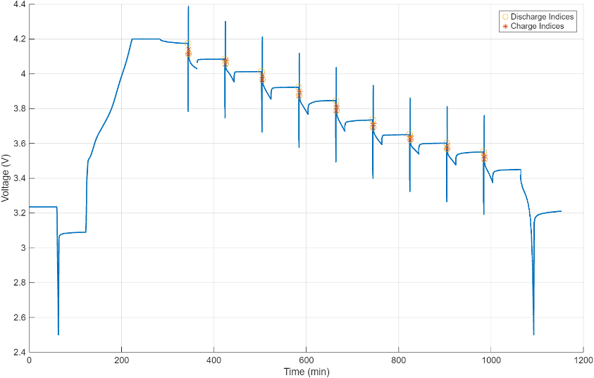
The plot shows all the identified charge and discharge pulse indices inside the
TestSummary property table of the hppcExp
object.
Input Arguments
Name-Value Arguments
Output Arguments
Version History
Introduced in R2025aSee Also
hppcTest | updateTestSummary | setDischargeSOCs | setChargeSOCs | removePulse | addPulseData | plotPulse

