Create Complex Baseband-Equivalent Model

Baseband-Equivalent Modeling

RF Blockset™ Equivalent Baseband software simulates the physical system in the time domain using a complex baseband-equivalent model that it creates from the passband frequency-domain parameters of the physical blocks. This type of modeling is also known as lowpass equivalent (LPE), complex envelope, or envelope modeling.

To create a complex baseband-equivalent model in the time domain based on the network parameters of the physical system, the blockset performs a mathematical transformation that consists of the following three steps:

1. Calculate the Passband Transfer Function

2. Calculate the Baseband-Equivalent Transfer Function

3. Calculate the Baseband-Equivalent Impulse Response

Calculate the Passband Transfer Function

The blockset calculates the passband transfer function from the physical block parameters at the modeling frequencies by calculating the transfer function of the physical subsystem and then applying the Tukey window to obtain the passband transfer function.

Note

To learn how the blockset uses the specified network parameters to compute the network parameters at the modeling frequencies, see Map Network Parameters to Modeling Frequencies.

The transfer function of the physical subsystem is defined as:

$$H(f)=\frac{V_L(f)}{V_S(f)}$$

where V_S and V_L are the source and load voltages shown in the following figure, and f represents the modeling frequencies.

More specifically,

$$H(f)=\frac{S_{21}\left(1+{\Gamma }_l\right)\left(1-{\Gamma }_s\right)}{2\left(1-S_{22}{\Gamma }_l\right)\left(1-{\Gamma }_{in}{\Gamma }_s\right)}$$

where

$$\begin{array}{l}{\Gamma }_l=\frac{Z_l-Z_o}{Z_l+Z_o}\\ {\Gamma }_s=\frac{Z_s-Z_o}{Z_s+Z_o}\\ {\Gamma }_{in}=S_{11}+\left(S_{12}{S}_{21}\frac{{\Gamma }_l}{\left(1-S_{22}{\Gamma }_l\right)}\right)\end{array}$$

and

• Z_S is the source impedance.

• Z_L is the load impedance.

• S_ij are the S-parameters of a two-port network.

The blockset derives the transfer function of the physical subsystem from the Input Port block parameters as shown in the following figure.

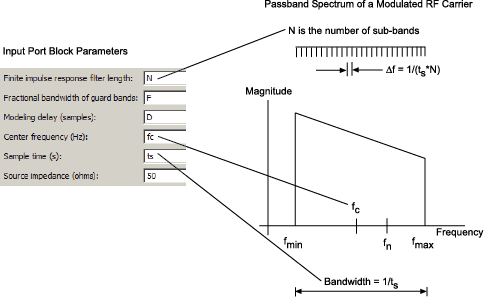
The blockset then applies the Tukey window to obtain the passband transfer function:

$$H_{passband}(f)=H(f)\cdot tukeywin(N,F)$$

where tukeywin is the Signal Processing Toolbox™ tukeywin (Signal Processing Toolbox) function.

Calculate the Baseband-Equivalent Transfer Function

The blockset calculates the baseband transfer function, $$H_{baseband}(f)$$, by translating the passband transfer function to its equivalent baseband transfer function:

$$H_{baseband}(f)=H_{passband}(f+f_c)$$

where f_c is the specified center frequency.

The resulting baseband-equivalent spectrum is centered at zero, so the blockset can simulate the system using a much larger time step than Simulink^® can use for the same system. For information on why this translation allows for a larger time step, see Simulation Efficiency of a Baseband-Equivalent Model.

The baseband transfer function is shown in the following figure.

Calculate the Baseband-Equivalent Impulse Response

The blockset calculates the baseband-equivalent impulse response by performing the following steps:

1. Calculate the inverse FFT of the baseband transfer function. For faster simulation, the block calculates the IFFT using the next power of 2 greater than the specified finite impulse response filter length. Then, it truncates the impulse response to a length equal to the filter length specified. When the finite impulse response is truncated to the length specified by the user, the effect of the truncation is similar to windowing with a rectangular window.

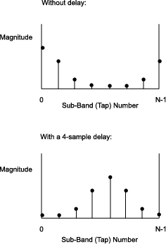
2. Apply the delay specified by the Modeling delay (samples) parameter in the Input Port block dialog box. Selecting an appropriate value for this delay ensures that the baseband-equivalent model has a causal response by moving the time window such that the model energy is concentrated at the center of the window, as shown in the following figure:

   

Simulation Efficiency of a Baseband-Equivalent Model

The baseband-equivalent modeling technique improves simulation speed by allowing the simulator to take larger time steps. To simulate a system in the time domain, Simulink would require a step size of:

$$t_{step}=\frac{1}{2f_{\max }}$$

Using the baseband-equivalent model of the same system, whose spectrum has been shifted down by f_c, allows for a much larger time step of:

$$t_{step}=\frac{1}{2(f_{\max }-f_c)}=\frac{1}{f_{\max }-f_{\min }}$$

Example — Select Parameter Values for a Baseband-Equivalent Model

• Baseband-Equivalent Modeling Example Overview

• Create the Model

• Specify Model Parameters

• Run the Simulation and Analyze the Results

• Reducing Acausal Response in the Baseband-Equivalent Model

• Introduce Delay into the Baseband-Equivalent Model

Baseband-Equivalent Modeling Example Overview

In this example, you model an RF transmission line stimulated by a pulse and plot the baseband-equivalent model that the blockset uses to simulate the transmission line in the time domain. You compare the effects of using different parameter values for the baseband-equivalent model. This example helps you understand how to use these parameters to best apply the baseband-equivalent modeling paradigm of performing time-domain simulation using a limited band of frequency data.

Create the Model

In this part of the example, you perform the following tasks:

• Select Blocks to Represent System Components

• Build the Model

• Specify Model Variables

Select Blocks to Represent System Components.  In this part of the example, you select the blocks to represent:

• The input signal

• The RF transmission line

• The baseband-equivalent model display

The following table lists the blocks that represent the system components and a description of the role of each block.

Block	Description
Discrete Impulse	Generates a frame-based pulse input signal.
Real-Imag to Complex	Converts the real pulse signal into a complex pulse signal.
Input Port	Establishes parameters that are common to all blocks in the RF transmission line subsystem, including the source impedance of the subsystem that is used to convert Simulink signals to the physical modeling environment.
RLCG Transmission Line	Models the signal attenuation caused by an RF transmission line.
Output Port	Establishes parameters that are common to all blocks in the RF transmission line subsystem. These parameters include the load impedance of the subsystem, which is used to convert RF signals to Simulink signals.
Complex to Magnitude-Angle	Converts the complex signal from the Output Port block into magnitude-angle format.

Build the Model.  In this part of the example, you create a Simulink model, add blocks to the model, and connect the blocks.

1. Create a model.

2. Add to the model the blocks shown in the following table. The Library Path column of the table specifies the hierarchical path to each block.

   Block	Library Path	Quantity
   Discrete Impulse	DSP System Toolbox > Sources	1
   Real-Imag to Complex	Simulink > Math Operations	1
   Input Port	RF Blockset > Equivalent Baseband > Input/Output Ports	1
   RLCG Transmission Line	RF Blockset > Equivalent Baseband > Transmission Lines	1
   Output Port	RF Blockset > Equivalent Baseband > Input/Output Ports	1
   Complex to Magnitude-Angle	Simulink > Math Operations	1

3. Connect the blocks as shown in the following figure.

   

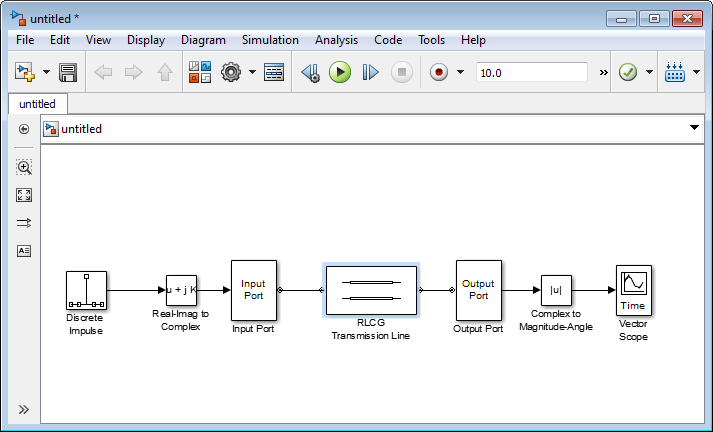
Now you are ready to specify model variables.

Specify Model Variables.  Type the following at the MATLAB^® prompt to set up workspace variables for the model:

t_s = 5e-10;   % Sample time
f_c = 3e9;	     % Center frequency
taps = 64;     % Filter length

Now you are ready to specify the block parameters.

Specify Model Parameters

In this part of the example, you specify the following parameters to represent the behavior of the system components:

• Input Signal Parameters

• Transmission Line Subsystem Parameters

• Signal Display Parameters

Input Signal Parameters.  You generate the frame-based complex pulse source signal using two blocks:

• The Discrete Impulse (DSP System Toolbox) block generates a real pulse signal.

• The Real-Imag to Complex block converts the real signal to a complex signal.

Note

All signals in the RF model must be complex to match the signals in the physical subsystem, so you create a complex input signal.

1. In the Discrete Impulse block parameters dialog box:

   • Set Sample time to t_s.

   • Set Samples per frame to 2*taps.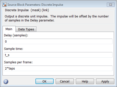

     

2. Set the Real-Imag to Complex block Input parameter to Real. Changing this parameter changes the number of block inputs from two to one, making the block fully connected.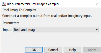

   

Transmission Line Subsystem Parameters.  In this part of the example, you configure the blocks that model the RF filter subsystem—the Input Port, Transmission Line, and Output Port blocks.

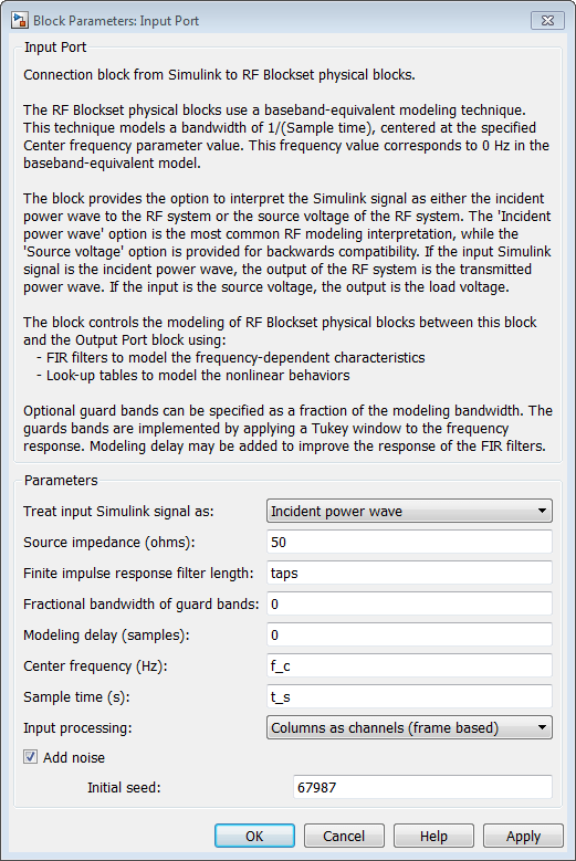
1. In the Input Port block parameters dialog box:

   • Set Treat input Simulink signal as to Incident power wave.

     This option tells the blockset to interpret the input signal as the incident power wave to the RF subsystem, and not the source voltage of the RF subsystem.

     Note

     If you use the default value for this parameter, the software interprets the input Simulink signal as the source voltage. As a result, the source and the load that model the Input Port and Output Port blocks, respectively, introduce 6 dB of loss into the physical system at all frequencies. For more information on why this loss occurs, see the note in Convert to and from Simulink Signals.

   • Set Finite impulse response filter length to taps.

   • Set Center frequency to f_c.

   • Set Sample time (s) to t_s.

     This sample time is equivalent to a modeling bandwidth of 1/t_s seconds.

   • Set Input Processing to Columns as channels (frame based).

   

2. In the RLCG Transmission Line block parameters dialog box:

   • Set Inductance per length (H/m) to 50.

   • Set Capacitance per length (F/m) to .02.

   • Set Frequency (Hz) to f_c.

   • Set Transmission line length (m) to 0.5*t_s.

   

3. Accept the default parameters for the Output Port block to use a load impedance of 50 ohms.

   

Signal Display Parameters.  In this part of the example, you specify the parameters that set up the baseband-equivalent model display. You use the Complex to Magnitude-Angle block to convert the RF subsystem output to magnitude format.

1. Set the Complex to Magnitude-Angle block Output parameter to Magnitude. Changing this parameter changes the number of block outputs from two to one, making the block fully connected.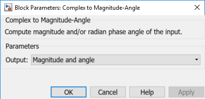

   

Run the Simulation and Analyze the Results

Before you run the simulation, set the stop time. Click Simulation In the PREPARE, click Model Settings in Configuration and Simulation. Enter 2*t_s*(taps-1) for the Stop time parameter.

To run the simulation, click Run in the model window.

This window appears automatically when you start the simulation. The following plot shows the baseband-equivalent model, which contains a significant amount of acausal energy because of the limited bandwidth of the model.

Baseband-Equivalent Model

The next part of the example shows you how to reduce this acausal response.

Reducing Acausal Response in the Baseband-Equivalent Model

In this part of the example, you adjust the Fractional bandwidth of guard bands parameter. This parameter controls the shaping of the filter that the blockset applies to create the baseband-equivalent model.

1. Set the Input Port Fractional bandwidth of guard bands parameter to 0.2.

2. Rerun the simulation.

You can see that the acausal response is lower than it was for the previous simulation, but there is still some energy wrapping around the end of the model because it is periodic.

Baseband-Equivalent Model with Filter Shaping

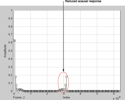
Note

You can further reduce the acausal response in the baseband-equivalent model by increasing the value of the Fractional bandwidth of guard bands parameter above 0.2, but if you use a high value, you compromise the fidelity of the gain of the transmission line.

The next section shows you how to shift the response to avoid this wrapping.

Introduce Delay into the Baseband-Equivalent Model

In this part of the example, you adjust the Modeling delay (samples) parameter. This parameter controls the delay the blockset applies to create the baseband-equivalent model.

1. Set the Input Port Modeling delay (samples) parameter to 12.

2. Rerun the simulation.

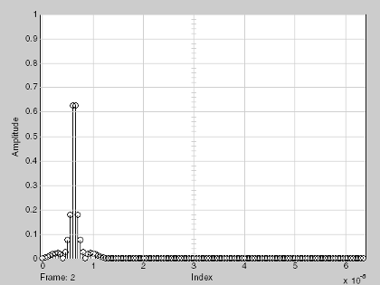
The response of the baseband-equivalent model is concentrated in a small time window. This model provides the most accurate time-domain simulation of the specified band of frequency data.

Baseband-Equivalent Model with Filter Shaping and Delay