Optimize SimEvents Models by Running Multiple Simulations
To optimize models in workflows that involve running multiple simulations, you can
create simulation tests using the Simulink.SimulationInput object.
Grocery Store Model
The grocery store example uses multiple simulations approach to optimize the number of shopping carts required to prevent long customer waiting lines.

In this example, the Entity Generator block represents the customer entry to the store. The customers wait in line if necessary and get a shopping cart through the Resource Acquirer block. The Resource Pool block represents the available shopping carts in the store. The Entity Server block represents the time each customer spends in the store. The customers return the shopping carts through the Resource Releaser block, while the Entity Terminator block represents customer departure from the store. The Average wait, w statistic from the Resource Acquirer block is saved to the workspace by the To Workspace block from the Simulink® library.
Build the Model
Grocery store customers wait in line if there are not enough shopping carts.
However, having too many unused shopping carts is considered a waste. The goal of
the example is to investigate the average customer wait time for a varying number of
available shopping carts in the store. To compute the average customer wait time,
multiple simulations are run by using the sim command. For each simulation, a
single available shopping cart value is used. For more information on the
sim command, see Run Parallel Simulations.
In the simulations, the available shopping cart value ranges from
20 to 50 and in each simulation it
increases by 1. It is assumed that during the operational hours,
customers arrive at the store with a random rate drawn from an exponential
distribution and their shopping duration is drawn from a uniform
distribution.
In the Entity Generator block, set the Entity type name to
Customersand the Time source toMATLAB action. Then, enter this code.persistent rngInit; if isempty(rngInit) seed = 12345; rng(seed); rngInit = true; end % Pattern: Exponential distribution mu = 1; dt = -mu*log(1-rand());
The time between the customer arrivals is drawn from an exponential distribution with mean
1minute.In the Resource Pool block, specify the Resource name as
ShoppingCart. Set the Resource amount to20.Initial value of available shopping carts is
20.In the Resource Acquirer block, set the
ShoppingCartas the Selected Resources, and set the Maximum number of waiting entities toInf.The example assumes a limitless number of customers who can wait for a shopping cart.
In the Entity Server block, set the Capacity to
Inf.The example assumes a limitless number of customers who can shop in the store.
In the Entity Server block, set the Service time source to
MATLAB actionand enter the code below.persistent rngInit; if isempty(rngInit) seed = 123456; rng(seed); rngInit = true; end % Pattern: Uniform distribution % m: Minimum, M: Maximum m = 20; M = 40; dt = m+(M-m)*rand;
The time a customer spends in the store is drawn from a uniform distribution on the interval between
20minutes and40minutes.Connect the Average wait, w statistic from the Resource Acquirer block to a To Workspace block and set its Variable name to
AverageCustomerWait.Set the simulation time to
600.The duration of one simulation is
10hours of operation which is600minutes.Save the model.
For this example, the model is saved with the name
GroceryStore_ShoppingCartExample.
Run Multiple Simulations to Optimize Resources
Open a new MATLAB® script and run this MATLAB code for multiple simulations.
Initialize the model and the available number of shopping carts for each simulation, which determines the number of simulations.
% Initialize the Grocery Store model with
% random intergeneration time and service time value
mdl = 'GroceryStore_ShoppingCartExample';
isModelOpen = bdIsLoaded(mdl);
open_system(mdl);

% Range of number of shopping carts that is
% used in each simulation
ShoppingCartNumber_Sweep = (20:1:50);
NumSims = length(ShoppingCartNumber_Sweep);
In each simulation, number of available shopping carts is increased by
1.Run each simulation with the corresponding available shopping cart value and output the results.
% Run NumSims number of simulations
NumCustomer = zeros(1,NumSims);
for i = 1:1:NumSims
    in(i) = Simulink.SimulationInput(mdl);
    % Use one ShoppingCartNumber_sweep value for each iteration
    in(i) = setBlockParameter(in(i), [mdl '/Resource Pool'], ...
    'ResourceAmount', num2str(ShoppingCartNumber_Sweep(i)));
end

% Output the results for each simulation
out = sim(in);
Gather and visualize the results.
% Compute maximum average wait time for the
% customers for each simulation
MaximumWait = zeros(1,NumSims);
for i=1:NumSims
    MaximumWait(i) = max(out(1, i).AverageCustomerWait.Data);
end
% Visualize the plot
plot(ShoppingCartNumber_Sweep, MaximumWait,'bo');
grid on
xlabel('Number of Available Shopping Carts')
ylabel('Maximum Wait Time')
Observe the plot that displays the maximum average wait time for the customers as a function of available shopping carts.
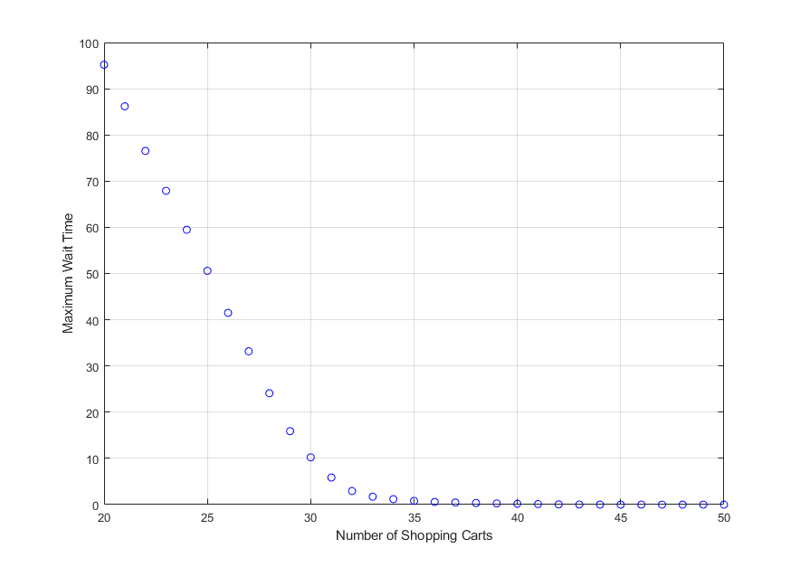
The plot displays the tradeoff between having
46shopping carts available for zero wait time versus33shopping carts for a2-minute customer wait time.
See Also
Entity Server | Entity Generator | Queue | Resource Acquirer | Entity Terminator | Resource Releaser | Resource Pool
Topics
- Optimization of Shared Resources in a Batch Production Process
- Explore Statistics and Visualize Simulation Results
- Interpret SimEvents Models Using Statistical Analysis
- Count Entities
- Visualization and Animation for Debugging
- Adjust Entity Generation Times Through Feedback
- Save SimEvents Simulation Operating Point