sbiofit

Perform nonlinear least-squares regression

Statistics and Machine Learning Toolbox™, Optimization Toolbox™, and Global Optimization Toolbox are recommended for this function.

Syntax

fitResults = sbiofit(sm,grpData,ResponseMap,estiminfo)

fitResults = sbiofit(sm,grpData,ResponseMap,estiminfo,dosing)

fitResults = sbiofit(sm,grpData,ResponseMap,estiminfo,dosing,functionName)

fitResults = sbiofit(sm,grpData,ResponseMap,estiminfo,dosing,functionName,options)

fitResults = sbiofit(sm,grpData,ResponseMap,estiminfo,dosing,functionName,options,variants)

fitResults = sbiofit(_,Name,Value)

[fitResults,simdata] = sbiofit(_)

Description

fitResults = sbiofit(sm,grpData,ResponseMap,estiminfo) estimates parameters of a SimBiology model sm using nonlinear least-squares regression.

grpData is a groupedData object specifying the data to fit. ResponseMap defines the mapping between the model components and response data in grpData. estimatedInfo is an EstimatedInfo object that defines the estimated parameters in the model sm. fitResults is a OptimResults object or NLINResults object or a vector of these objects.

sbiofit uses the first available estimation function among the following: lsqnonlin (Optimization Toolbox), nlinfit (Statistics and Machine Learning Toolbox), or fminsearch.

By default, each group in grpData is fit separately, resulting in group-specific parameter estimates. If the model contains active doses and variants, they are applied before the simulation.

fitResults = sbiofit(sm,grpData,ResponseMap,estiminfo,dosing) uses the dosing information specified by a matrix of SimBiology dose objects dosing instead of using the active doses of the model sm if there is any.

fitResults = sbiofit(sm,grpData,ResponseMap,estiminfo,dosing,functionName) uses the estimation function specified by functionName. If the specified function is unavailable, a warning is issued and the first available default function is used.

fitResults = sbiofit(sm,grpData,ResponseMap,estiminfo,dosing,functionName,options) uses the additional options specified by options for the function functionName.

fitResults = sbiofit(sm,grpData,ResponseMap,estiminfo,dosing,functionName,options,variants) applies variant objects specified as variants instead of using any active variants of the model.

fitResults = sbiofit(_,Name,Value) uses additional options specified by one or more Name,Value pair arguments.

[fitResults,simdata] = sbiofit(_) also returns a vector of SimData objects simdata using any of the input arguments in the previous syntaxes.

Note

• sbiofit unifies sbionlinfit and sbioparamestim estimation functions. Use sbiofit to perform nonlinear least-squares regression.

• sbiofit simulates the model using a SimFunction object, which automatically accelerates simulations by default. Hence it is not necessary to run sbioaccelerate before you call sbiofit.

Examples

Fit One-Compartment Model to Individual PK Profile

Background

This example shows how to fit an individual's PK profile data to one-compartment model and estimate pharmacokinetic parameters.

Suppose you have drug plasma concentration data from an individual and want to estimate the volume of the central compartment and the clearance. Assume the drug concentration versus the time profile follows the monoexponential decline $$C_t=C_0{e}^{-k_{e}t}$$, where $$C_t$$ is the drug concentration at time t, $$C_0$$ is the initial concentration, and $$k_e$$ is the elimination rate constant that depends on the clearance and volume of the central compartment $$k_e=Cl/V$$.

The synthetic data in this example was generated using the following model, parameters, and dose:

• One-compartment model with bolus dosing and first-order elimination

• Volume of the central compartment (Central) = 1.70 liter

• Clearance parameter (Cl_Central) = 0.55 liter/hour

• Constant error model

• Bolus dose of 10 mg

Load Data and Visualize

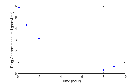
The data is stored as a table with variables Time and Conc that represent the time course of the plasma concentration of an individual after an intravenous bolus administration measured at 13 different time points. The variable units for Time and Conc are hour and milligram/liter, respectively.

load('data15.mat')
plot(data.Time,data.Conc,'b+')
xlabel('Time (hour)');
ylabel('Drug Concentration (milligram/liter)');

Convert to groupedData Format

Convert the data set to a groupedData object, which is the required data format for the fitting function sbiofit for later use. A groupedData object also lets you set independent variable and group variable names (if they exist). Set the units of the Time and Conc variables. The units are optional and only required for the UnitConversion feature, which automatically converts matching physical quantities to one consistent unit system.

gData = groupedData(data);
gData.Properties.VariableUnits = {'hour','milligram/liter'};
gData.Properties

ans = struct with fields:
                Description: ''
                   UserData: []
             DimensionNames: {'Row'  'Variables'}
              VariableNames: {'Time'  'Conc'}
              VariableTypes: ["double"    "double"]
       VariableDescriptions: {}
              VariableUnits: {'hour'  'milligram/liter'}
         VariableContinuity: []
                   RowNames: {}
           CustomProperties: [1×1 matlab.tabular.CustomProperties]
          GroupVariableName: ''
    IndependentVariableName: 'Time'

groupedData automatically set the name of the IndependentVariableName property to the Time variable of the data.

Construct a One-Compartment Model

Use the built-in PK library to construct a one-compartment model with bolus dosing and first-order elimination where the elimination rate depends on the clearance and volume of the central compartment. Use the configset object to turn on unit conversion.

pkmd                    = PKModelDesign;
pkc1                    = addCompartment(pkmd,'Central');
pkc1.DosingType         = 'Bolus';
pkc1.EliminationType    = 'linear-clearance';
pkc1.HasResponseVariable = true;
model                   = construct(pkmd);
configset               = getconfigset(model);
configset.CompileOptions.UnitConversion = true;

For details on creating compartmental PK models using the SimBiology® built-in library, see Create Pharmacokinetic Models.

Define Dosing

Define a single bolus dose of 10 milligram given at time = 0. For details on setting up different dosing schedules, see Doses in SimBiology Models.

dose                = sbiodose('dose');
dose.TargetName     = 'Drug_Central';
dose.StartTime      = 0;
dose.Amount         = 10;
dose.AmountUnits    = 'milligram';
dose.TimeUnits      = 'hour';

Map Response Data to the Corresponding Model Component

The data contains drug concentration data stored in the Conc variable. This data corresponds to the Drug_Central species in the model. Therefore, map the data to Drug_Central as follows.

responseMap = {'Drug_Central = Conc'};

Specify Parameters to Estimate

The parameters to fit in this model are the volume of the central compartment (Central) and the clearance rate (Cl_Central). In this case, specify log-transformation for these biological parameters since they are constrained to be positive. The estimatedInfo object lets you specify parameter transforms, initial values, and parameter bounds if needed.

paramsToEstimate    = {'log(Central)','log(Cl_Central)'};
estimatedParams     = estimatedInfo(paramsToEstimate,'InitialValue',[1 1],'Bounds',[1 5;0.5 2]);

Estimate Parameters

Now that you have defined one-compartment model, data to fit, mapped response data, parameters to estimate, and dosing, use sbiofit to estimate parameters. The default estimation function that sbiofit uses will change depending on which toolboxes are available. To see which function was used during fitting, check the EstimationFunction property of the corresponding results object.

fitConst = sbiofit(model,gData,responseMap,estimatedParams,dose);

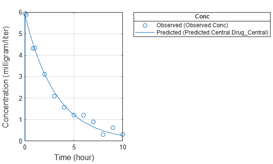
Display Estimated Parameters and Plot Results

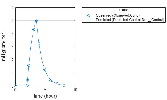
Notice the parameter estimates were not far off from the true values (1.70 and 0.55) that were used to generate the data. You may also try different error models to see if they could further improve the parameter estimates.

fitConst.ParameterEstimates

ans=2×4 table
         Name         Estimate    StandardError      Bounds  
    ______________    ________    _____________    __________

    {'Central'   }     1.6993       0.034821         1      5
    {'Cl_Central'}    0.53358        0.01968       0.5      2

s.Labels.XLabel     = 'Time (hour)';
s.Labels.YLabel     = 'Concentration (milligram/liter)';
plot(fitConst,'AxesStyle',s);

Use Different Error Models

Try three other supported error models (proportional, combination of constant and proportional error models, and exponential).

fitProp = sbiofit(model,gData,responseMap,estimatedParams,dose,...
                      'ErrorModel','proportional');
fitExp  = sbiofit(model,gData,responseMap,estimatedParams,dose,...
                      'ErrorModel','exponential');
fitComb = sbiofit(model,gData,responseMap,estimatedParams,dose,...
                      'ErrorModel','combined');

Use Weights Instead of an Error Model

You can specify weights as a numeric matrix, where the number of columns corresponds to the number of responses. Setting all weights to 1 is equivalent to the constant error model.

weightsNumeric = ones(size(gData.Conc));
fitWeightsNumeric = sbiofit(model,gData,responseMap,estimatedParams,dose,'Weights',weightsNumeric);

Alternatively, you can use a function handle that accepts a vector of predicted response values and returns a vector of weights. In this example, use a function handle that is equivalent to the proportional error model.

weightsFunction = @(y) 1./y.^2;
fitWeightsFunction = sbiofit(model,gData,responseMap,estimatedParams,dose,'Weights',weightsFunction);

Compare Information Criteria for Model Selection

Compare the loglikelihood, AIC, and BIC values of each model to see which error model best fits the data. A larger likelihood value indicates the corresponding model fits the model better. For AIC and BIC, the smaller values are better.

allResults = [fitConst,fitWeightsNumeric,fitWeightsFunction,fitProp,fitExp,fitComb];
errorModelNames = {'constant error model','equal weights','proportional weights', ...
                   'proportional error model','exponential error model',...
                   'combined error model'};
LogLikelihood = [allResults.LogLikelihood]';
AIC = [allResults.AIC]';
BIC = [allResults.BIC]';
t = table(LogLikelihood,AIC,BIC);
t.Properties.RowNames = errorModelNames;
t

t=6×3 table
                                LogLikelihood      AIC        BIC  
                                _____________    _______    _______

    constant error model            3.9866       -3.9732    -2.8433
    equal weights                   3.9866       -3.9732    -2.8433
    proportional weights           -3.8472        11.694     12.824
    proportional error model       -3.8257        11.651     12.781
    exponential error model         1.1984        1.6032     2.7331
    combined error model            3.9163       -3.8326    -2.7027

Based on the information criteria, the constant error model (or equal weights) fits the data best since it has the largest loglikelihood value and the smallest AIC and BIC.

Display Estimated Parameter Values

Show the estimated parameter values of each model.

Estimated_Central       = zeros(6,1);
Estimated_Cl_Central    = zeros(6,1);
t2 = table(Estimated_Central,Estimated_Cl_Central);
t2.Properties.RowNames = errorModelNames;
for i = 1:height(t2)
    t2{i,1} = allResults(i).ParameterEstimates.Estimate(1);
    t2{i,2} = allResults(i).ParameterEstimates.Estimate(2);
end
t2

t2=6×2 table
                                Estimated_Central    Estimated_Cl_Central
                                _________________    ____________________

    constant error model             1.6993                0.53358       
    equal weights                    1.6993                0.53358       
    proportional weights             1.9045                0.51734       
    proportional error model         1.8777                0.51147       
    exponential error model          1.7872                0.51701       
    combined error model             1.7008                0.53271       

Conclusion

This example showed how to estimate PK parameters, namely the volume of the central compartment and clearance parameter of an individual, by fitting the PK profile data to one-compartment model. You compared the information criteria of each model and estimated parameter values of different error models to see which model best explained the data. Final fitted results suggested both the constant and combined error models provided the closest estimates to the parameter values used to generate the data. However, the constant error model is a better model as indicated by the loglikelihood, AIC, and BIC information criteria.

Fit Two-Compartment Model to PK Profiles of Multiple Individuals

Suppose you have drug plasma concentration data from three individuals that you want to use to estimate corresponding pharmacokinetic parameters, namely the volume of central and peripheral compartment (Central, Peripheral), the clearance rate (Cl_Central), and intercompartmental clearance (Q12). Assume the drug concentration versus the time profile follows the biexponential decline $$C_t=A{e}^{-at}+B{e}^{-bt}$$, where C_t is the drug concentration at time t, and a and b are slopes for corresponding exponential declines.

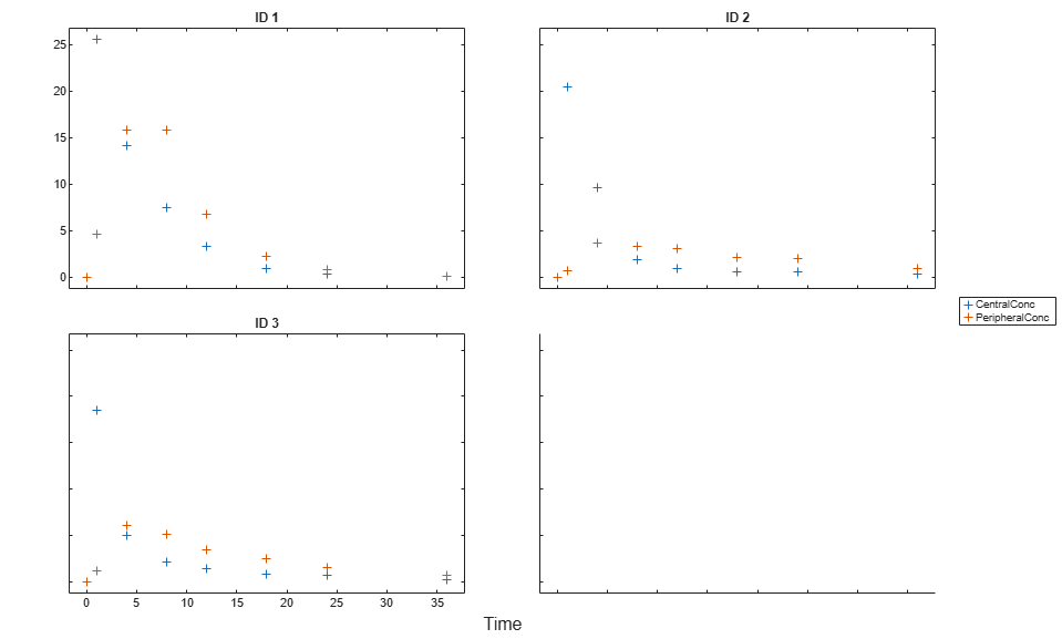
The synthetic data set contains drug plasma concentration data measured in both central and peripheral compartments. The data was generated using a two-compartment model with an infusion dose and first-order elimination. These parameters were used for each individual.

	Central	Peripheral	Q12	Cl_Central
Individual 1	1.90	0.68	0.24	0.57
Individual 2	2.10	6.05	0.36	0.95
Individual 3	1.70	4.21	0.46	0.95

The data is stored as a table with variables ID, Time, CentralConc, and PeripheralConc. It represents the time course of plasma concentrations measured at eight different time points for both central and peripheral compartments after an infusion dose.

load('data10_32R.mat')

Convert the data set to a groupedData object which is the required data format for the fitting function sbiofit for later use. A groupedData object also lets you set independent variable and group variable names (if they exist). Set the units of the ID, Time, CentralConc, and PeripheralConc variables. The units are optional and only required for the UnitConversion feature, which automatically converts matching physical quantities to one consistent unit system.

gData = groupedData(data);
gData.Properties.VariableUnits = {'','hour','milligram/liter','milligram/liter'};
gData.Properties

ans = 

  struct with fields:

                Description: ''
                   UserData: []
             DimensionNames: {'Row'  'Variables'}
              VariableNames: {'ID'  'Time'  'CentralConc'  'PeripheralConc'}
              VariableTypes: ["double"    "double"    "double"    "double"]
       VariableDescriptions: {}
              VariableUnits: {''  'hour'  'milligram/liter'  'milligram/liter'}
         VariableContinuity: []
                   RowNames: {}
           CustomProperties: [1×1 matlab.tabular.CustomProperties]
          GroupVariableName: 'ID'
    IndependentVariableName: 'Time'

Create a trellis plot that shows the PK profiles of three individuals.

sbiotrellis(gData,'ID','Time',{'CentralConc','PeripheralConc'},...
            'Marker','+','LineStyle','none');

Use the built-in PK library to construct a two-compartment model with infusion dosing and first-order elimination where the elimination rate depends on the clearance and volume of the central compartment. Use the configset object to turn on unit conversion.

pkmd                 = PKModelDesign;
pkc1                 = addCompartment(pkmd,'Central');
pkc1.DosingType      = 'Infusion';
pkc1.EliminationType = 'linear-clearance';
pkc1.HasResponseVariable = true;
pkc2                 = addCompartment(pkmd,'Peripheral');
model                = construct(pkmd);
configset            = getconfigset(model);
configset.CompileOptions.UnitConversion = true;

Assume every individual receives an infusion dose at time = 0, with a total infusion amount of 100 mg at a rate of 50 mg/hour. For details on setting up different dosing strategies, see Doses in SimBiology Models.

dose             = sbiodose('dose','TargetName','Drug_Central');
dose.StartTime   = 0;
dose.Amount      = 100;
dose.Rate        = 50;
dose.AmountUnits = 'milligram';
dose.TimeUnits   = 'hour';
dose.RateUnits   = 'milligram/hour';

The data contains measured plasma concentrations in the central and peripheral compartments. Map these variables to the appropriate model species, which are Drug_Central and Drug_Peripheral.

responseMap = {'Drug_Central = CentralConc','Drug_Peripheral = PeripheralConc'};

The parameters to estimate in this model are the volumes of central and peripheral compartments (Central and Peripheral), intercompartmental clearance Q12, and clearance rate Cl_Central. In this case, specify log-transform for Central and Peripheral since they are constrained to be positive. The estimatedInfo object lets you specify parameter transforms, initial values, and parameter bounds (optional).

paramsToEstimate   = {'log(Central)','log(Peripheral)','Q12','Cl_Central'};
estimatedParam     = estimatedInfo(paramsToEstimate,'InitialValue',[1 1 1 1]);

Fit the model to all of the data pooled together, that is, estimate one set of parameters for all individuals. The default estimation method that sbiofit uses will change depending on which toolboxes are available. To see which estimation function sbiofit used for the fitting, check the EstimationFunction property of the corresponding results object.

pooledFit = sbiofit(model,gData,responseMap,estimatedParam,dose,'Pooled',true)

pooledFit = 

  OptimResults with properties:

                   ExitFlag: 3
                     Output: [1×1 struct]
                  GroupName: []
                       Beta: [4×3 table]
         ParameterEstimates: [4×3 table]
                          J: [24×4×2 double]
                       COVB: [4×4 double]
           CovarianceMatrix: [4×4 double]
                          R: [24×2 double]
                        MSE: 6.6220
                        SSE: 291.3688
                    Weights: []
              LogLikelihood: -111.3904
                        AIC: 230.7808
                        BIC: 238.2656
                        DFE: 44
             DependentFiles: {1×3 cell}
                       Data: [24×4 groupedData]
    EstimatedParameterNames: {'Central'  'Peripheral'  'Q12'  'Cl_Central'}
             ErrorModelInfo: [1×3 table]
         EstimationFunction: 'lsqnonlin'

Plot the fitted results versus the original data. Although three separate plots were generated, the data was fitted using the same set of parameters (that is, all three individuals had the same fitted line).

plot(pooledFit);

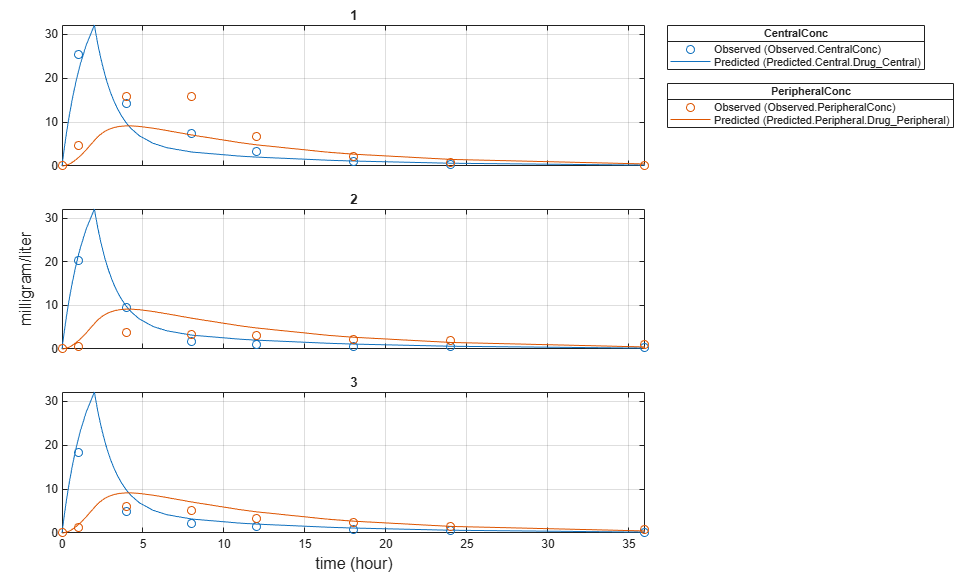
Estimate one set of parameters for each individual and see if there is any improvement in the parameter estimates. In this example, since there are three individuals, three sets of parameters are estimated.

unpooledFit =  sbiofit(model,gData,responseMap,estimatedParam,dose,'Pooled',false);

Plot the fitted results versus the original data. Each individual was fitted differently (that is, each fitted line is unique to each individual) and each line appeared to fit well to individual data.

plot(unpooledFit);

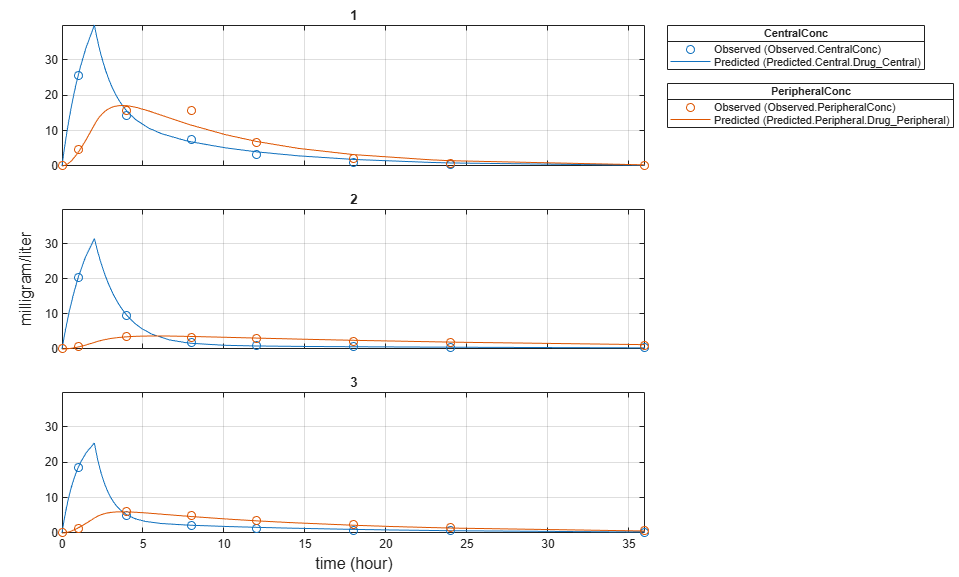
Display the fitted results of the first individual. The MSE was lower than that of the pooled fit. This is also true for the other two individuals.

unpooledFit(1)

ans = 

  OptimResults with properties:

                   ExitFlag: 3
                     Output: [1×1 struct]
                  GroupName: 1
                       Beta: [4×3 table]
         ParameterEstimates: [4×3 table]
                          J: [8×4×2 double]
                       COVB: [4×4 double]
           CovarianceMatrix: [4×4 double]
                          R: [8×2 double]
                        MSE: 2.1380
                        SSE: 25.6559
                    Weights: []
              LogLikelihood: -26.4805
                        AIC: 60.9610
                        BIC: 64.0514
                        DFE: 12
             DependentFiles: {1×3 cell}
                       Data: [8×4 groupedData]
    EstimatedParameterNames: {'Central'  'Peripheral'  'Q12'  'Cl_Central'}
             ErrorModelInfo: [1×3 table]
         EstimationFunction: 'lsqnonlin'

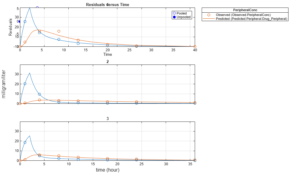
Generate a plot of the residuals over time to compare the pooled and unpooled fit results. The figure indicates unpooled fit residuals are smaller than those of pooled fit as expected. In addition to comparing residuals, other rigorous criteria can be used to compare the fitted results.

t = [gData.Time;gData.Time];
res_pooled = vertcat(pooledFit.R);
res_pooled = res_pooled(:);
res_unpooled = vertcat(unpooledFit.R);
res_unpooled = res_unpooled(:);
plot(t,res_pooled,'o','MarkerFaceColor','w','markerEdgeColor','b')
hold on
plot(t,res_unpooled,'o','MarkerFaceColor','b','markerEdgeColor','b')
refl = refline(0,0); % A reference line representing a zero residual
title('Residuals versus Time');
xlabel('Time');
ylabel('Residuals');
legend({'Pooled','Unpooled'});

This example showed how to perform pooled and unpooled estimations using sbiofit. As illustrated, the unpooled fit accounts for variations due to the specific subjects in the study, and, in this case, the model fits better to the data. However, the pooled fit returns population-wide parameters. If you want to estimate population-wide parameters while considering individual variations, use sbiofitmixed.

Estimate Category-Specific PK Parameters for Multiple Individuals

This example shows how to estimate category-specific (such as young versus old, male versus female), individual-specific, and population-wide parameters using PK profile data from multiple individuals.

Background

Suppose you have drug plasma concentration data from 30 individuals and want to estimate pharmacokinetic parameters, namely the volumes of central and peripheral compartment, the clearance, and intercompartmental clearance. Assume the drug concentration versus the time profile follows the biexponential decline $$C_t=A{e}^{-at}+B{e}^{-bt}$$, where $$C_t$$ is the drug concentration at time t, and $$a$$ and $$b$$ are slopes for corresponding exponential declines.

Load Data

This synthetic data contains the time course of plasma concentrations of 30 individuals after a bolus dose (100 mg) measured at different times for both central and peripheral compartments. It also contains categorical variables, namely Sex and Age.

clear
load('sd5_302RAgeSex.mat')

Convert to groupedData Format

Convert the data set to a groupedData object, which is the required data format for the fitting function sbiofit. A groupedData object also allows you set independent variable and group variable names (if they exist). Set the units of the ID, Time, CentralConc, PeripheralConc, Age, and Sex variables. The units are optional and only required for the UnitConversion feature, which automatically converts matching physical quantities to one consistent unit system.

gData = groupedData(data);
gData.Properties.VariableUnits = {'','hour','milligram/liter','milligram/liter','',''};
gData.Properties

ans = struct with fields:
                Description: ''
                   UserData: []
             DimensionNames: {'Row'  'Variables'}
              VariableNames: {'ID'  'Time'  'CentralConc'  'PeripheralConc'  'Sex'  'Age'}
              VariableTypes: ["double"    "double"    "double"    "double"    "categorical"    "categorical"]
       VariableDescriptions: {}
              VariableUnits: {''  'hour'  'milligram/liter'  'milligram/liter'  ''  ''}
         VariableContinuity: []
                   RowNames: {}
           CustomProperties: [1×1 matlab.tabular.CustomProperties]
          GroupVariableName: 'ID'
    IndependentVariableName: 'Time'

The IndependentVariableName and GroupVariableName properties have been automatically set to the Time and ID variables of the data.

Visualize Data

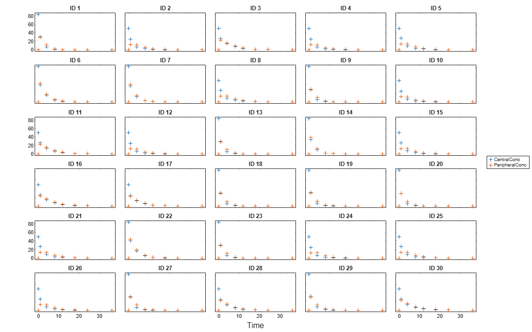
Display the response data for each individual.

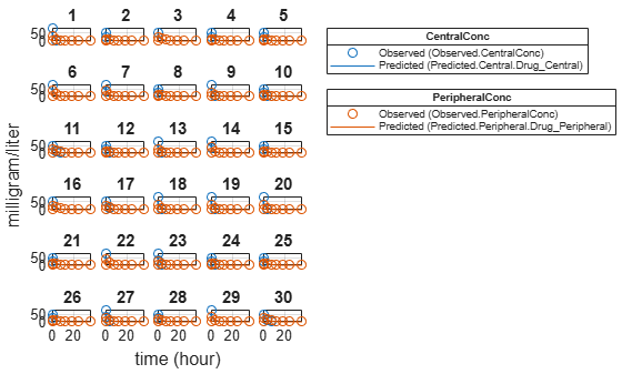
t = sbiotrellis(gData,'ID','Time',{'CentralConc','PeripheralConc'},...
                'Marker','+','LineStyle','none');
% Resize the figure.
t.hFig.Position(:) = [100 100 1280 800];

Set Up a Two-Compartment Model

Use the built-in PK library to construct a two-compartment model with infusion dosing and first-order elimination where the elimination rate depends on the clearance and volume of the central compartment. Use the configset object to turn on unit conversion.

pkmd                                    = PKModelDesign;
pkc1                                    = addCompartment(pkmd,'Central');
pkc1.DosingType                         = 'Bolus';
pkc1.EliminationType                    = 'linear-clearance';
pkc1.HasResponseVariable                = true;
pkc2                                    = addCompartment(pkmd,'Peripheral');
model                                   = construct(pkmd);
configset                               = getconfigset(model);
configset.CompileOptions.UnitConversion = true;

For details on creating compartmental PK models using the SimBiology® built-in library, see Create Pharmacokinetic Models.

Define Dosing

Assume every individual receives a bolus dose of 100 mg at time = 0. For details on setting up different dosing strategies, see Doses in SimBiology Models.

dose             = sbiodose('dose','TargetName','Drug_Central');
dose.StartTime   = 0;
dose.Amount      = 100;
dose.AmountUnits = 'milligram';
dose.TimeUnits   = 'hour';

Map the Response Data to Corresponding Model Components

The data contains measured plasma concentration in the central and peripheral compartments. Map these variables to the appropriate model components, which are Drug_Central and Drug_Peripheral.

responseMap = {'Drug_Central = CentralConc','Drug_Peripheral = PeripheralConc'};

Specify Parameters to Estimate

Specify the volumes of central and peripheral compartments Central and Peripheral, intercompartmental clearance Q12, and clearance Cl_Central as parameters to estimate. The estimatedInfo object lets you optionally specify parameter transforms, initial values, and parameter bounds. Since both Central and Peripheral are constrained to be positive, specify a log-transform for each parameter.

paramsToEstimate    = {'log(Central)', 'log(Peripheral)', 'Q12', 'Cl_Central'};
estimatedParam      = estimatedInfo(paramsToEstimate,'InitialValue',[1 1 1 1]);

Estimate Individual-Specific Parameters

Estimate one set of parameters for each individual by setting the 'Pooled' name-value pair argument to false.

unpooledFit =  sbiofit(model,gData,responseMap,estimatedParam,dose,'Pooled',false);

Display Results

Plot the fitted results versus the original data for each individual (group).

plot(unpooledFit);

For an unpooled fit, sbiofit always returns one results object for each individual.

Examine Parameter Estimates for Category Dependencies

Explore the unpooled estimates to see if there is any category-specific parameters, that is, if some parameters are related to one or more categories. If there are any category dependencies, it might be possible to reduce the number of degrees of freedom by estimating just category-specific values for those parameters.

First extract the ID and category values for each ID

catParamValues = unique(gData(:,{'ID','Sex','Age'}));

Add variables to the table containing each parameter's estimate.

allParamValues            = vertcat(unpooledFit.ParameterEstimates);
catParamValues.Central    = allParamValues.Estimate(strcmp(allParamValues.Name, 'Central'));
catParamValues.Peripheral = allParamValues.Estimate(strcmp(allParamValues.Name, 'Peripheral'));
catParamValues.Q12        = allParamValues.Estimate(strcmp(allParamValues.Name, 'Q12'));
catParamValues.Cl_Central = allParamValues.Estimate(strcmp(allParamValues.Name, 'Cl_Central'));

Plot estimates of each parameter for each category. gscatter requires Statistics and Machine Learning Toolbox™. If you do not have it, use other alternative plotting functions such as plot.

h           = figure;
ylabels     = ["Central","Peripheral","Q12","Cl\_Central"];
plotNumber  = 1;
for i = 1:4
    thisParam = estimatedParam(i).Name;
    
    % Plot for Sex category
    subplot(4,2,plotNumber);
    plotNumber  = plotNumber + 1;
    gscatter(double(catParamValues.Sex), catParamValues.(thisParam), catParamValues.Sex);
    ax          = gca;
    ax.XTick    = [];
    ylabel(ylabels(i));
    legend('Location','bestoutside')
    % Plot for Age category
    subplot(4,2,plotNumber);
    plotNumber  = plotNumber + 1;
    gscatter(double(catParamValues.Age), catParamValues.(thisParam), catParamValues.Age);
    ax          = gca;
    ax.XTick    = [];
    ylabel(ylabels(i));
    legend('Location','bestoutside')
end
% Resize the figure.
h.Position(:) = [100 100 1280 800];

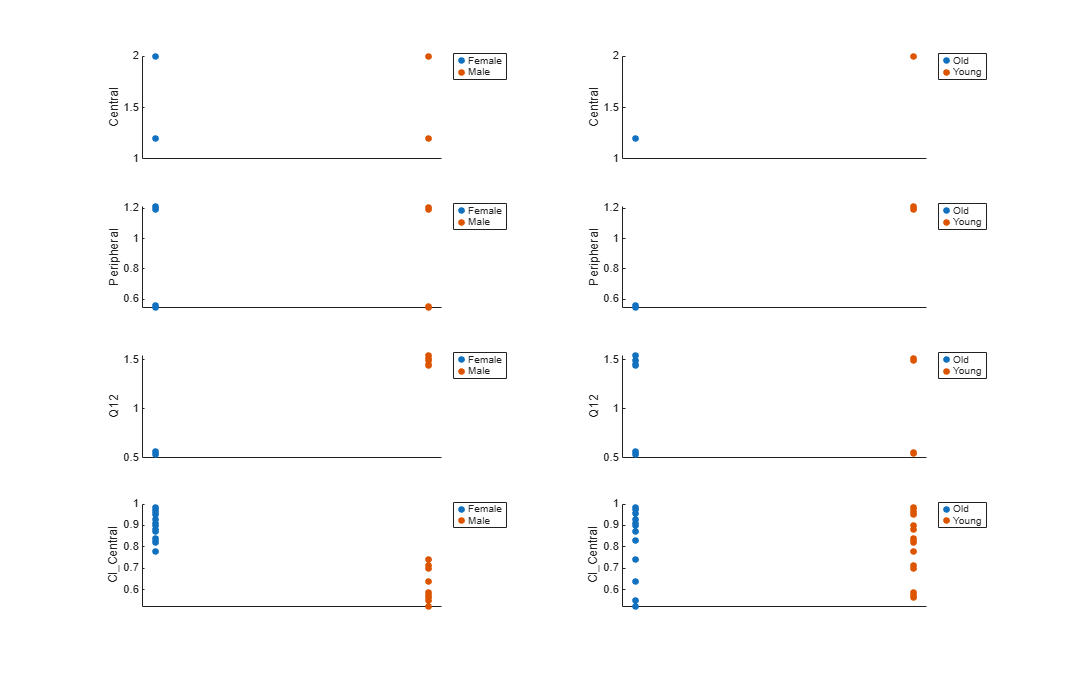
Based on the plot, it seems that young individuals tend to have higher volumes of central and peripheral compartments (Central, Peripheral) than old individuals (that is, the volumes seem to be age-specific). In addition, males tend to have lower clearance rates (Cl_Central) than females but the opposite for the Q12 parameter (that is, the clearance and Q12 seem to be sex-specific).

Estimate Category-Specific Parameters

Use the 'CategoryVariableName' property of the estimatedInfo object to specify which category to use during fitting. Use 'Sex' as the group to fit for the clearance Cl_Central and Q12 parameters. Use 'Age' as the group to fit for the Central and Peripheral parameters.

estimatedParam(1).CategoryVariableName = 'Age';
estimatedParam(2).CategoryVariableName = 'Age';
estimatedParam(3).CategoryVariableName = 'Sex';
estimatedParam(4).CategoryVariableName = 'Sex';
categoryFit = sbiofit(model,gData,responseMap,estimatedParam,dose)

categoryFit = 
  OptimResults with properties:

                   ExitFlag: 3
                     Output: [1×1 struct]
                  GroupName: []
                       Beta: [8×5 table]
         ParameterEstimates: [120×6 table]
                          J: [240×8×2 double]
                       COVB: [8×8 double]
           CovarianceMatrix: [8×8 double]
                          R: [240×2 double]
                        MSE: 0.4362
                        SSE: 205.8690
                    Weights: []
              LogLikelihood: -477.9195
                        AIC: 971.8390
                        BIC: 1.0052e+03
                        DFE: 472
             DependentFiles: {1×3 cell}
                       Data: [240×6 groupedData]
    EstimatedParameterNames: {'Central'  'Peripheral'  'Q12'  'Cl_Central'}
             ErrorModelInfo: [1×3 table]
         EstimationFunction: 'lsqnonlin'

When fitting by category (or group), sbiofit always returns one results object, not one for each category level. This is because both male and female individuals are considered to be part of the same optimization using the same error model and error parameters, similarly for the young and old individuals.

Plot Results

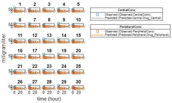
Plot the category-specific estimated results.

plot(categoryFit);

For the Cl_Central and Q12 parameters, all males had the same estimates, and similarly for the females. For the Central and Peripheral parameters, all young individuals had the same estimates, and similarly for the old individuals.

Estimate Population-Wide Parameters

To better compare the results, fit the model to all of the data pooled together, that is, estimate one set of parameters for all individuals by setting the 'Pooled' name-value pair argument to true. The warning message tells you that this option will ignore any category-specific information (if they exist).

pooledFit = sbiofit(model,gData,responseMap,estimatedParam,dose,'Pooled',true);

Warning: CategoryVariableName property of the estimatedInfo object is ignored when using the 'Pooled' option.

Plot Results

Plot the fitted results versus the original data. Although a separate plot was generated for each individual, the data was fitted using the same set of parameters (that is, all individuals had the same fitted line).

plot(pooledFit);

Compare Residuals

Compare residuals of CentralConc and PeripheralConc responses for each fit.

t = gData.Time;
allResid(:,:,1) = pooledFit.R;
allResid(:,:,2) = categoryFit.R;
allResid(:,:,3) = vertcat(unpooledFit.R);

h = figure;
responseList = {'CentralConc', 'PeripheralConc'};
for i = 1:2
    subplot(2,1,i);
    oneResid = squeeze(allResid(:,i,:));
    plot(t,oneResid,'o');
    refline(0,0); % A reference line representing a zero residual
    title(sprintf('Residuals (%s)', responseList{i}));
    xlabel('Time');
    ylabel('Residuals');
    legend({'Pooled','Category-Specific','Unpooled'});
end
% Resize the figure.
h.Position(:) = [100 100 1280 800];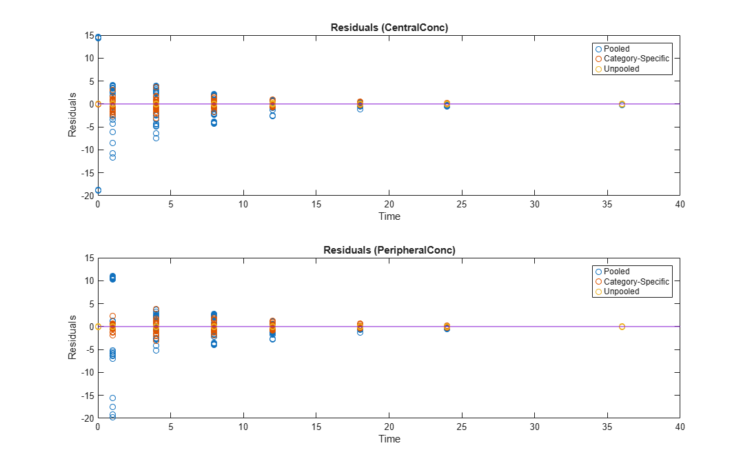

As shown in the plot, the unpooled fit produced the best fit to the data as it fit the data to each individual. This was expected since it used the most number of degrees of freedom. The category-fit reduced the number of degrees of freedom by fitting the data to two categories (sex and age). As a result, the residuals were larger than the unpooled fit, but still smaller than the population-fit, which estimated just one set of parameters for all individuals. The category-fit might be a good compromise between the unpooled and pooled fitting provided that any hierarchical model exists within your data.

Estimate Yeast G Protein Model Parameter

This example uses the yeast heterotrimeric G protein model and experimental data reported by [1]. For details about the model, see the Background section in Parameter Scanning, Parameter Estimation, and Sensitivity Analysis in the Yeast Heterotrimeric G Protein Cycle.

Load the G protein model.

sbioloadproject gprotein

Store the experimental data containing the time course for the fraction of active G protein.

time = [0 10 30 60 110 210 300 450 600]';
GaFracExpt = [0 0.35 0.4 0.36 0.39 0.33 0.24 0.17 0.2]';

Create a groupedData object based on the experimental data.

tbl = table(time,GaFracExpt);
grpData = groupedData(tbl);

Map the appropriate model component to the experimental data. In other words, indicate which species in the model corresponds to which response variable in the data. In this example, map the model parameter GaFrac to the experimental data variable GaFracExpt from grpData.

responseMap = 'GaFrac = GaFracExpt';

Use an estimatedInfo object to define the model parameter kGd as a parameter to be estimated.

estimatedParam = estimatedInfo('kGd');

Perform the parameter estimation.

fitResult = sbiofit(m1,grpData,responseMap,estimatedParam);

View the estimated parameter value of kGd.

fitResult.ParameterEstimates

ans=1×3 table
     Name      Estimate    StandardError
    _______    ________    _____________

    {'kGd'}    0.11307      3.4439e-05  

Suppose you want to plot the model simulation results using the estimated parameter value. You can either rerun the sbiofit function and specify to return the optional second output argument, which contains simulation results, or use the fitted method to retrieve the results without rerunning sbiofit.

[yfit,paramEstim] = fitted(fitResult);

Plot the simulation results.

sbioplot(yfit);

Estimate Time Lag and Duration of a Dose

This example shows how to estimate the time lag before a bolus dose was administered and the duration of the dose using a one-compartment model.

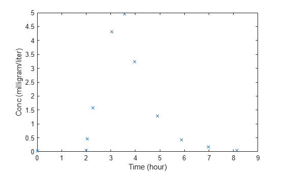
Load a sample data set.

load lagDurationData.mat

Plot the data.

plot(data.Time,data.Conc,'x')
xlabel('Time (hour)')
ylabel('Conc (milligram/liter)')

Convert to groupedData.

gData = groupedData(data);
gData.Properties.VariableUnits = {'hour','milligram/liter'};

Create a one-compartment model.

pkmd                    = PKModelDesign;
pkc1                    = addCompartment(pkmd,'Central');
pkc1.DosingType         = 'Bolus';
pkc1.EliminationType    = 'linear-clearance';
pkc1.HasResponseVariable = true;
model                   = construct(pkmd);
configset               = getconfigset(model);
configset.CompileOptions.UnitConversion = true;

Add two parameters that represent the time lag and duration of a dose. The lag parameter specifies the time lag before the dose is administered. The duration parameter specifies the length of time it takes to administer a dose.

lagP = addparameter(model,'lagP');
lagP.ValueUnits = 'hour';
durP = addparameter(model,'durP');
durP.ValueUnits = 'hour';

Create a dose object. Set the LagParameterName and DurationParameterName properties of the dose to the names of the lag and duration parameters, respectively. Set the dose amount to 10 milligram which was the amount used to generate the data.

dose                = sbiodose('dose');
dose.TargetName     = 'Drug_Central';
dose.StartTime      = 0;
dose.Amount         = 10;
dose.AmountUnits    = 'milligram';
dose.TimeUnits      = 'hour';
dose.LagParameterName = 'lagP';
dose.DurationParameterName = 'durP';

Map the model species to the corresponding data.

responseMap = {'Drug_Central = Conc'};

Specify the lag and duration parameters as parameters to estimate. Log-transform the parameters. Initialize them to 2 and set the upper bound and lower bound.

paramsToEstimate    = {'log(lagP)','log(durP)'};
estimatedParams     = estimatedInfo(paramsToEstimate,'InitialValue',2,'Bounds',[1 5]);

Perform parameter estimation.

fitResults = sbiofit(model,gData,responseMap,estimatedParams,dose,'fminsearch')

fitResults = 
  OptimResults with properties:

                   ExitFlag: 1
                     Output: [1×1 struct]
                  GroupName: One group
                       Beta: [2×4 table]
         ParameterEstimates: [2×4 table]
                          J: [11×2 double]
                       COVB: [2×2 double]
           CovarianceMatrix: [2×2 double]
                          R: [11×1 double]
                        MSE: 0.0024
                        SSE: 0.0213
                    Weights: []
              LogLikelihood: 18.7511
                        AIC: -33.5023
                        BIC: -32.7065
                        DFE: 9
             DependentFiles: {1×2 cell}
                       Data: [11×2 groupedData]
    EstimatedParameterNames: {'lagP'  'durP'}
             ErrorModelInfo: [1×3 table]
         EstimationFunction: 'fminsearch'

Display the result.

fitResults.ParameterEstimates

ans=2×4 table
      Name      Estimate    StandardError    Bounds
    ________    ________    _____________    ______

    {'lagP'}     1.986        0.0051568      1    5
    {'durP'}     1.527         0.012956      1    5

plot(fitResults)

Use Group-Specific Dosing Data for Parameter Estimation with Numeric Weights

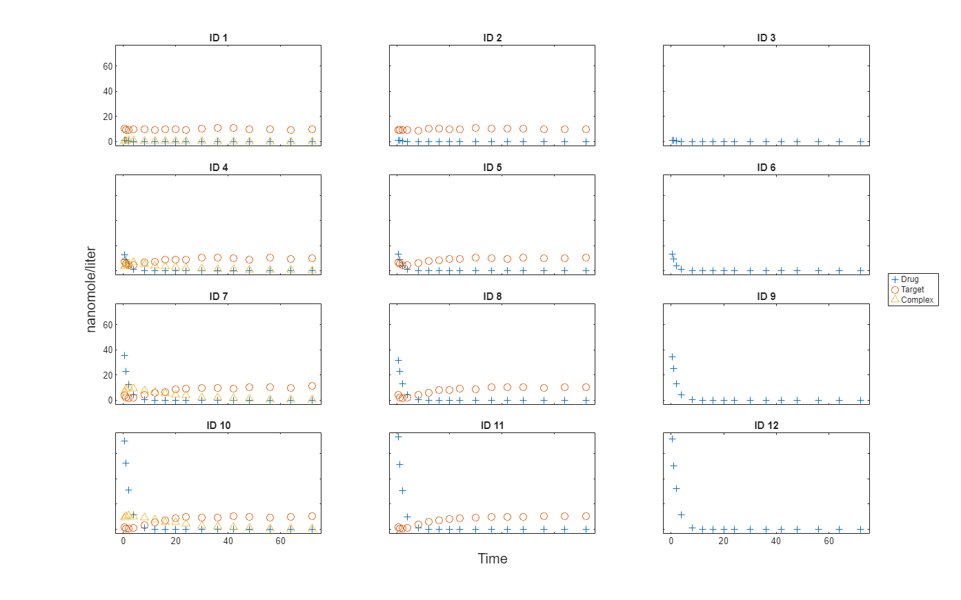
Import data to use for fitting. It comprises 12 groups of measurements across three responses: Drug, Target, and Complex. The Drug response includes measurements for all 12 groups, whereas the Target and Complex responses have measurements for only 8 and 4 groups, respectively. A group could represent a patient or an experimental or biological condition. Ndrug, Ntarget, and Ncomplex columns represent the constant number of groups that have the measurements for the corresponding responses. Each group has its own dosing amount, represented by the Dose column.

dataTMDD = readtable('tmddData_final.csv');

Display the first few rows of the data set.

head(dataTMDD)

    ID    Time    Dose      Drug       Target    Complex    Ndrug    Ntarget    Ncomplex
    __    ____    ____    _________    ______    _______    _____    _______    ________

    1       0      10           NaN       NaN        NaN     12         8          4    
    1     0.5     NaN        1.2131    10.116    0.36602     12         8          4    
    1       1     NaN       0.74803    9.4694    0.61803     12         8          4    
    1       2     NaN       0.28601    9.2434    0.84304     12         8          4    
    1       4     NaN      0.048002    9.6184    0.83204     12         8          4    
    1       8     NaN     0.0080003    9.6334    0.67203     12         8          4    
    1      12     NaN     0.0060003    9.4574    0.54002     12         8          4    
    1      16     NaN     0.0050002    9.7914    0.40502     12         8          4    

Convert the data to a groupedData format.

gData = groupedData(dataTMDD);
gData.Properties.VariableUnits = ["","hour","nanomole","nanomole/liter","nanomole/liter","nanomole/liter","","",""];
gData.Properties.GroupVariableName = "ID";
gData.Properties.IndependentVariableName = "Time";

Plot the responses: Drug, Target, and Complex.

t = sbiotrellis(gData,"ID","Time","Drug",Marker="+",LineStyle="none"); 
plot(t,gData,"ID","Time","Target",Marker="o",LineStyle="none");
plot(t,gData,"ID","Time","Complex",Marker="^",LineStyle="none");
t.hFig.Position = [100 100 1280 800];
t.YLabel = "nanomole/liter";

Load the target-mediated drug deposition (TMDD) model. For details about the model, see Scan Dosing Regimens Using SimBiology Model Analyzer App.

sbioloadproject("tmdd_with_TO.sbproj","m1");

The data has 12 groups of measurements, and each group has its own dose amount. Create a corresponding dose object for each group using the dosing information from the data. During the subsequent fitting step, the fit function applies each dose to each group in the same order that the groups appear in the input data. For details on setting up doses, see dosing.

dose = sbiodose("Dose");
dose.TargetName = "Plasma.Drug";
doses = createDoses(gData,"Dose","",dose);

Specify parameters to estimate and their initial values. Also set upper and lower parameter bounds.

paramsToEstimate = estimatedInfo(["log(km)","log(kon)","log(koff)"],InitialValue=0.01,Bounds=[1e-05 1]);

Map the measurement data to the corresponding model components.

responseMap = ["Plasma.Drug = Drug",...
               "Plasma.Target = Target",...
               "Plasma.Complex = Complex"];

Define the algorithm options.

options                     = optimoptions("lsqnonlin");
options.StepTolerance       = 1e-08;
options.FunctionTolerance   = 1e-08;
options.OptimalityTolerance = 1e-06;
options.MaxIterations       = 100;

Define the fit problem.

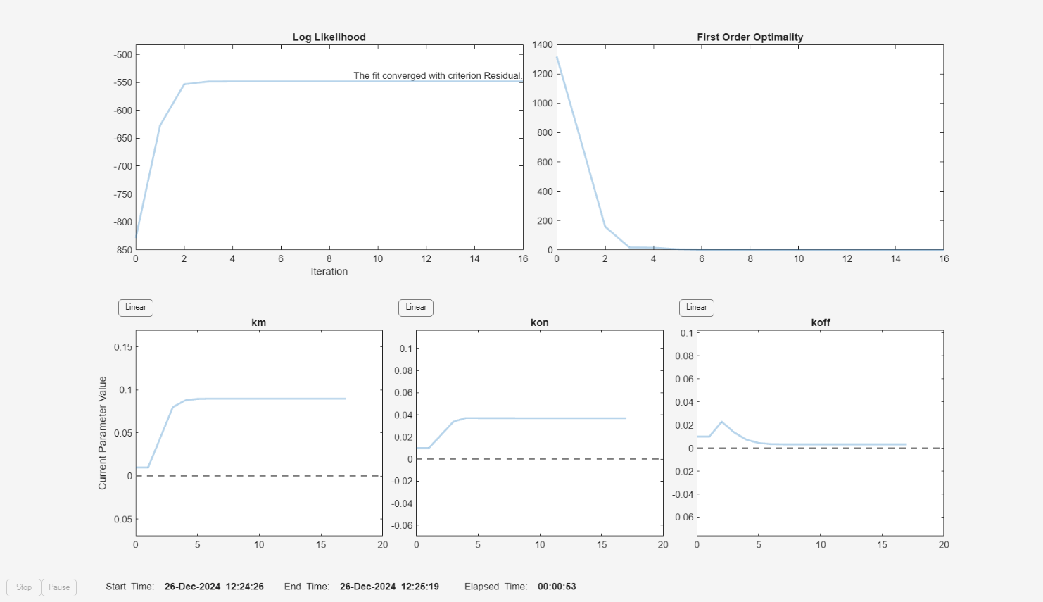
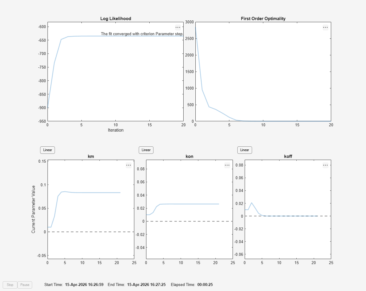
f              = fitproblem(FitFunction="sbiofit");
f.Data         = gData;
f.Estimated    = paramsToEstimate;
f.Model        = m1;
f.ResponseMap  = responseMap;

f.Doses        = doses;
f.FunctionName = "lsqnonlin";
f.Options      = options;
f.Pooled       = true;
f.ProgressPlot = true;

Run the fit with weights set to 1.

f.Weights = [ones(size(gData.Drug)) ones(size(gData.Target)) ones(size(gData.Complex))];
fitEqualWeights = fit(f);

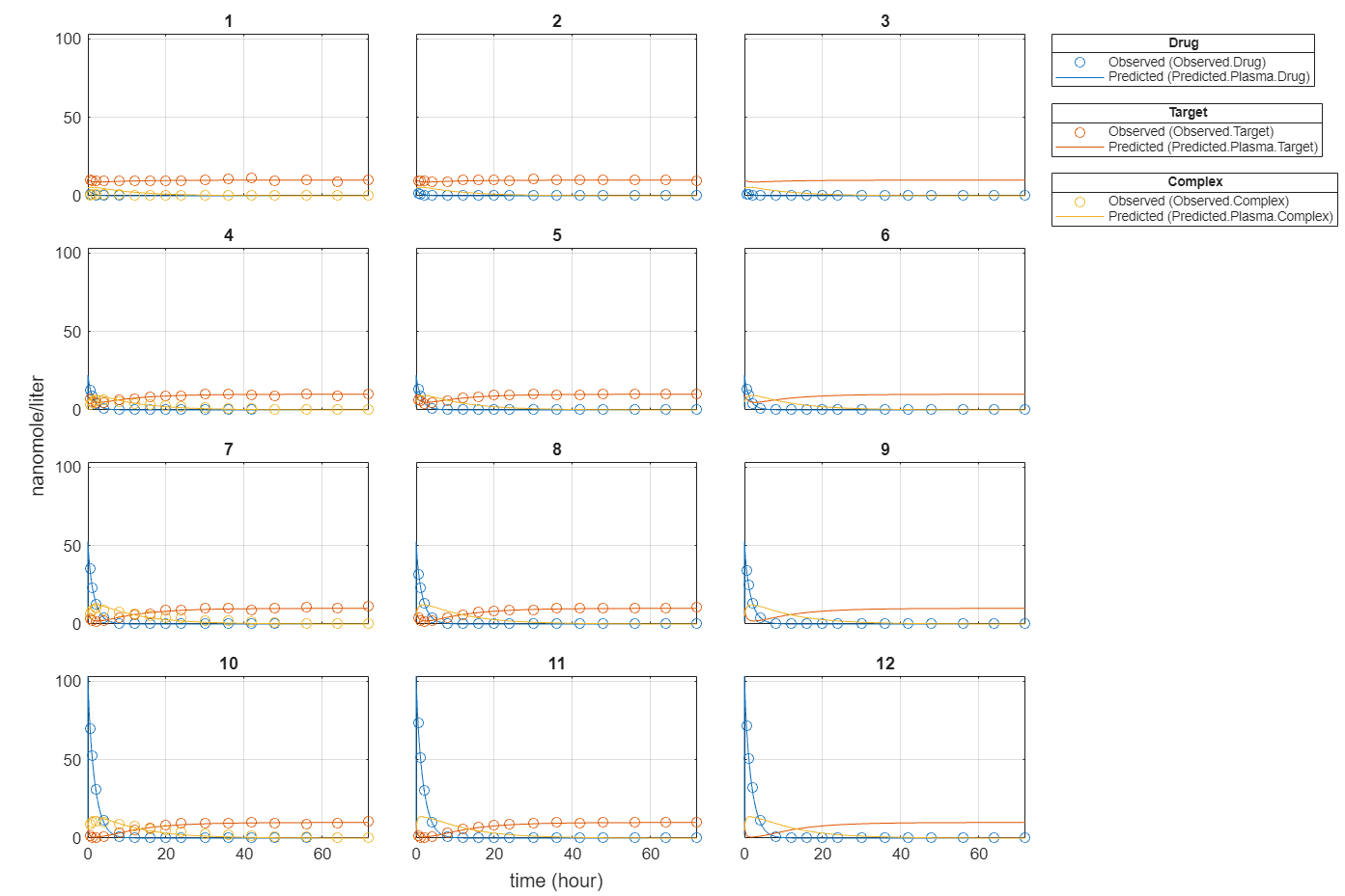
plot(fitEqualWeights);

Plot all groups in one plot for each response.

plot(fitEqualWeights,PlotStyle="one axes");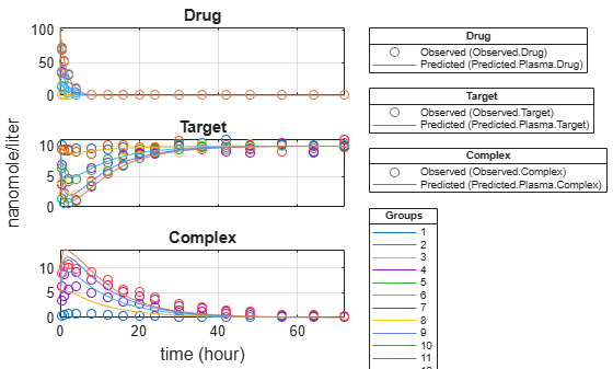

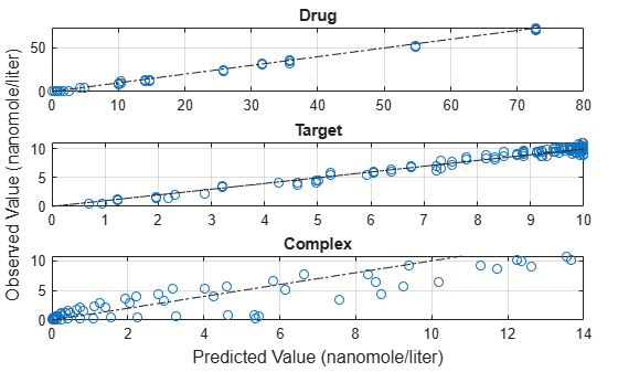
Compare the predictions to the actual data.

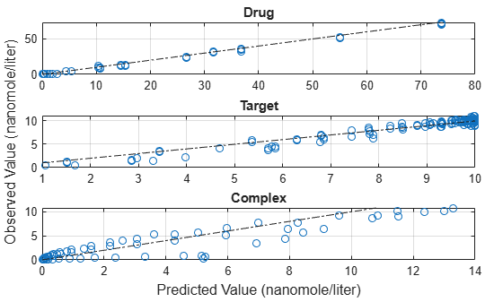
plotActualVersusPredicted(fitEqualWeights)

In this data set, the response Drug has 12 groups of measurements, Target has 8 groups of measurements, and Complex has 4 groups of measurements. The varying number of measurements among these responses might stem from the experimental design. To address these differences, you might consider experimenting with weights that are inversely proportional to the number of measurement groups.

f.Weights = [1./gData.Ndrug 1./gData.Ntarget 1./gData.Ncomplex];
fitInverseWeights = fit(f);

plot(fitInverseWeights);

Plot all groups in one plot for each response.

plot(fitInverseWeights,PlotStyle="one axes");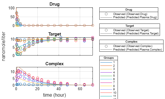

Compare the predictions to the actual data.

plotActualVersusPredicted(fitInverseWeights)

Input Arguments

sm — SimBiology model

SimBiology model object

SimBiology model, specified as a SimBiology model object. The active configset object of the model contains solver settings for simulation. Any active doses and variants are applied to the model during simulation unless specified otherwise using the dosing and variants input arguments, respectively.

grpData — Data to fit

groupedData object

Data to fit, specified as a groupedData object.

The name of the time variable must be defined in the IndependentVariableName property of grpData. For instance, if the time variable name is 'TIME', then specify it as follows.

grpData.Properties.IndependentVariableName = 'TIME';

If the data contains more than one group of measurements, the grouping variable name must be defined in the GroupVariableName property of grpData. For example, if the grouping variable name is 'GROUP', then specify it as follows.

grpData.Properties.GroupVariableName = 'GROUP';

A group usually refers to a set of measurements that represent a single time course, often corresponding to a particular individual, or experimental condition.

Note

sbiofit uses the categorical function to identify groups. If any group values are converted to the same value by categorical, then those observations are treated as belonging to the same group. For instance, if some observations have no group information (that is, an empty character vector ''), then categorical converts empty character vectors to <undefined>, and these observations are treated as one group.

ResponseMap — Mapping information of model components to grpData

character vector | string | string vector | cell array of character vectors

Mapping information of model components to grpData, specified as a character vector, string, string vector, or cell array of character vectors.

Each character vector or string is an equation-like expression, similar to assignment rules in SimBiology. It contains the name (or qualified name) of a quantity (species, compartment, or parameter) or an observable object in the model sm, followed by the character '=' and the name of a variable in grpData. For clarity, white spaces are allowed between names and '='.

For example, if you have the concentration data 'CONC' in grpData for a species 'Drug_Central', you can specify it as follows.

ResponseMap = 'Drug_Central = CONC';

To name a species unambiguously, use the qualified name, which includes the name of the compartment. To name a reaction-scoped parameter, use the reaction name to qualify the parameter.

If the model component name or grpData variable name is not a valid MATLAB^® variable name, surround it by square brackets, such as:

ResponseMap = '[Central 1].Drug = [Central 1 Conc]';

If a variable name itself contains square brackets, you cannot use it in the expression to define the mapping information.

An error is issued if any (qualified) name matches two components of the same type. However, you can use a (qualified) name that matches two components of different types, and the function first finds the species with the given name, followed by compartments and then parameters.

estiminfo — Estimated parameters

estimatedInfo object | vector of estimatedInfo objects

Estimated parameters, specified as an EstimatedInfo object or vector of estimatedInfo objects that defines the estimated parameters in the model sm, and other optional information such as their initial estimates, transformations, bound constraints, and categories. Supported transforms are log, logit, and probit. For details, see Parameter Transformations.

You can specify bounds for all estimation methods. The lower bound must be less than the upper bound. For details, see Bounds.

When using scattersearch, you must specify finite transformed bounds for each estimated parameter.

When using fminsearch, nlinfit, or fminunc with bounds, the objective function returns Inf if bounds are exceeded. When you turn on options such as FunValCheck, the optimization might error if bounds are exceeded during estimation. If using nlinfit, it might report warnings about the Jacobian being ill-conditioned or not being able to estimate if the final result is too close to the bounds.

If you do not specify Pooled name-value pair argument, sbiofit uses CategoryVariableName property of estiminfo to decide if parameters must be estimated for each individual, group, category, or all individuals as a whole. Use the Pooled option to override any CategoryVariableName values. For details about CategoryVariableName property, see EstimatedInfo object.

Note

sbiofit uses the categorical function to identify groups or categories. If any group values are converted to the same value by categorical, then those observations are treated as belonging to the same group. For instance, if some observations have no group information (that is, an empty character vector '' as a group value), then categorical converts empty character vectors to <undefined>, and these observations are treated as one group.

dosing — Dosing information

[] | {} | 2-D matrix of dose objects | cell vector of dose objects

Dosing information, specified as an empty array ([] or {}), 2-D matrix or cell vector of dose objects (ScheduleDose object or RepeatDose object).

If you omit the dosing input, the function applies the active doses of the model if there are any.

If you specify the input as empty [] or {}, no doses are applied during simulation, even if the model has active doses.

For a matrix of dose objects, it must have a single row or one row per group in the input data. If it has a single row, the same doses are applied to all groups during simulation. If it has multiple rows, each row is applied to a separate group, in the same order as the groups appear in the input data. Multiple columns are allowed so that you can apply multiple dose objects to each group.

Note

As of R2021b, doses in the columns are no longer required to have the same configuration. If you previously created default (dummy) doses to fill in the columns, these default doses have no effect and indicate no dosing.

For a cell vector of doses, it must have one element or one element per group in the input data. Each element must be [] or a vector of doses. Each element of the cell is applied to a separate group, in the same order as the groups appear in the input data.

In addition to manually constructing dose objects using sbiodose, if the input groupedData object has dosing information, you can use the createDoses method to construct doses.

functionName — Estimation function name

character vector | string

Estimation function name, specified as a character vector or string. Choices are as follows.

• "fminsearch"

• "nlinfit" (Statistics and Machine Learning Toolbox is required.)

• "fminunc" (Optimization Toolbox is required.)

• "fmincon" (Optimization Toolbox is required.)

• "lsqcurvefit" (Optimization Toolbox is required.)

• "lsqnonlin" (Optimization Toolbox is required.)

• "patternsearch" (Global Optimization Toolbox is required.)

• "ga" (Global Optimization Toolbox is required.)

• "particleswarm" (Global Optimization Toolbox is required.)

• "scattersearch"

By default, sbiofit uses the first available estimation function among the following: lsqnonlin (Optimization Toolbox), nlinfit (Statistics and Machine Learning Toolbox), or fminsearch. The same priority applies to the default local solver choice for scattersearch.

For the summary of supported methods and fitting options, see Supported Methods for Parameter Estimation in SimBiology.

options — Options specific to estimation function

struct | optimoptions object

Options specific to the estimation function, specified as a struct or optimoptions object.

• statset struct for nlinfit

• optimset struct for fminsearch

• optimoptions object for lsqcurvefit, lsqnonlin, fmincon, fminunc, particleswarm, ga, and patternsearch

• struct for scattersearch

See Default Options for Estimation Algorithms for more details and default options associated with each estimation function.

variants — Variants

[] | {} | vector of variant objects

Variants, specified as an empty array ([] or {}) or vector of variant objects.

If you

• Omit this input argument, the function applies the active variants of the model if there are any.

• Specify this input as empty, no variants are used even if the model has active variants.

• Specify this input as a vector of variants, the function applies the specified variants to all simulations, and the model active variants are not used.

• Specify this input as a vector of variants and also specify the Variants name-value argument, the function applies the variants specified in this input argument before applying the ones specified in the name-value argument.

Name-Value Arguments

Specify optional pairs of arguments as Name1=Value1,...,NameN=ValueN, where Name is the argument name and Value is the corresponding value. Name-value arguments must appear after other arguments, but the order of the pairs does not matter.

Example: fitResults = sbiofit(sm,grpData,ResponseMap,covEstiminfo,ErrorModel="proportional",UseParallel=true) specifies a proportional error model and to run simulations in parallel during parameter estimation.

ErrorModel — Error model

'constant' (default) | character vector | string | string vector | cell array of character vector | categorical vector | table

Error model to use for estimation, specified as a character vector, string scalar, string vector, cell array of character vectors, categorical vector, or table. Valid values are "constant", "proportional", "combined", and "exponential".

The following details apply:

• If you specify only one error model, then sbiofit estimates one set of error parameters for all responses.

• If you specify multiple error models using a categorical vector, string vector, or cell array of character vectors, the length of the vector or cell array must match the number of responses in ResponseMap.

• You can specify multiple error models only if you are using these methods: lsqnonlin, lsqcurvefit, fmincon, fminunc, fminsearch, patternsearch, ga, and particleswarm. For more details, see Maximum Likelihood Estimation.

• If you specify weights only for the constant error model.

• If you specify a table, it must contain a single variable that is a column vector of error model names. The names can be a cell array of character vectors, string vector, or a vector of categorical variables. If the table has more than one row and the RowNames property is not empty, then the RowNames property must match the response variable names specified in the right hand side of ResponseMap. If the table does not use the RowNames property, the nth error is associated with the nth response.

Four built-in error models are available. Each model defines the error using a standard mean-zero and unit-variance (Gaussian) variable e, simulation results f, and one or two parameters a and b.

• "constant": $$y=f+ae$$

• "proportional": $$y=f+b\left|f\right|e$$

• "combined": $$y=f+(a+b\left|f\right|)e$$

• "exponential": $$y=f\ast \exp (ae)$$

For more details, see Error Models.

Note

If you use a proportional or combined error model during data fitting, avoid specifying data points at times where the solution (simulation result) is zero or the steady state is zero. Otherwise, you can run into division-by-zero problems. To avoid those problems, remove those data points from the data set.

Weights — Weights used for fitting

[] (default) | matrix | function handle

Weights used for fitting, specified as an empty array [], matrix of real positive weights where the number of columns corresponds to the number of responses, or a function handle that accepts a vector of predicted response values and returns a vector of real positive weights.

If you specify an error model, you cannot use weights except for the constant error model. If neither the ErrorModel or Weights is specified, by default, the software uses the constant error model with equal weights.

Variants — Group-specific variants

[] | {} | 2-D matrix of variants | cell vector of variants

Group-specific variants, specified as an empty array ([] or {}), 2-D matrix or cell vector of variant objects. These variants let you specify parameter values for specific groups during fitting. The software applies these group-specific variants after active variants or the variants input argument. If the value is empty ([] or {}), no group-specific variants are applied.

For a matrix of variant objects, the number of rows must be one or must match the number of groups in the input data. The ith row of variant objects is applied to the simulation of the ith group. The variants are applied in order from the first column to the last. If this matrix has only one row of variants, they are applied to all simulations.

For a cell vector of variant objects, the number of cells must be one or must match the number of groups in the input data. Each element must be [] or a vector of variants. If this cell vector has a single cell containing a vector of variants, they are applied to all simulations. If the cell vector has multiple cells, the variants in the ith cell are applied to the simulation of the ith group.

In addition to manually constructing variant objects using sbiovariant, if the input groupedData object has variant information, you can use createVariants to construct variants.

Pooled — Fit option flag

false or 0 (default) | true or 1

Fit option flag to fit each individual or pool all individual data, specified as a numeric or logical 1 (true) or 0 (false).

When true, the software performs fitting for all individuals or groups simultaneously using the same parameter estimates, and fitResults is a scalar results object.

When false, the software fits each group or individual separately using group- or individual-specific parameters, and fitResults is a vector of results objects with one result for each group.

Note

Use this option to override any CategoryVariableName values of estiminfo.

UseParallel — Flag for parallel simulations

false or 0 (default) | true or 1

Flag to enable parallelization, specified as a numeric or logical 1 (true) or 0 (false). If true and Parallel Computing Toolbox™ is available, sbiofit supports several levels of parallelization, but only one level is used at a time.

For an unpooled fit (Pooled = false) for multiple groups, each fit is run in parallel.

For a pooled fit (Pooled = true), parallelization happens at the solver level. In other words, solver computations, such as objective function evaluations, are run in parallel.

For details, see Multiple Parameter Estimations in Parallel.

SensitivityAnalysis — Flag to use parameter sensitivities to determine gradients of the objective function

false or 0 (default) | true or 1

Flag to use parameter sensitivities to determine gradients of the objective function, specified as a numeric or logical 1 (true) or 0 (false). By default, it is true for fmincon, fminunc, lsqnonlin, lsqcurvefit, and scattersearch methods. Otherwise, it is false.

If it is true, the software always uses the sundials solver, regardless of what you have selected as the SolverType property in the Configset object.

The software uses the complex-step approximation method to calculate parameter sensitivities. Such calculated sensitivities can be used to determine gradients of the objective function during parameter estimation to improve fitting. The default behavior of sbiofit is to use such sensitivities to determine gradients whenever the algorithm is gradient-based and if the SimBiology model supports sensitivity analysis. For details about the model requirements and sensitivity analysis, see Sensitivity Analysis in SimBiology.

ProgressPlot — Flag to show the progress of parameter estimation

false or 0 (default) | true or 1

Flag to show the progress of parameter estimation, specified as a numeric or logical 1 (true) or 0 (false). If true, a new figure opens containing plots.

Plots show the log-likelihood, termination criteria, and estimated parameters for each iteration. This option is not supported for nlinfit.

If you are using the Optimization Toolbox functions (fminunc, fmincon, lsqcurvefit, lsqnonlin), the figure also shows the First Order Optimality (Optimization Toolbox) plot.

For an unpooled fit, each line on the plots represents an individual. For a pooled fit, a single line represents all individuals. The line becomes faded when the fit is complete. The plots also keep track of the progress when you run sbiofit (for both pooled and unpooled fits) in parallel using remote clusters. For details, see Progress Plot.

Output Arguments

fitResults — Estimation results

OptimResults object | NLINResults object | vector of results objects

Estimation results, returned as a OptimResults object or NLINResults object or a vector of these objects. Both results objects are subclasses of the LeastSquaresResults object.

If the function uses nlinfit (Statistics and Machine Learning Toolbox), then fitResults is a NLINResults object. Otherwise, fitResults is an OptimResults object.

For an unpooled fit, the function fits each group separately using group-specific parameters, and fitResults is a vector of results objects with one results object for each group.

For a pooled fit, the function performs fitting for all individuals or groups simultaneously using the same parameter estimates, and fitResults is a scalar results object.

When the pooled option is not specified, and CategoryVariableName values of estimatedInfo objects are all <none>, fitResults is a single results object. This is the same behavior as a pooled fit.

When the pooled option is not specified, and CategoryVariableName values of estimatedInfo objects are all <GroupVariableName>, fitResults is a vector of results objects. This is the same behavior as an unpooled fit.

In all other cases, fitResults is a scalar object containing estimated parameter values for different groups or categories specified by CategoryVariableName.

simdata — Simulation results

vector of SimData objects

Simulation results, returned as a vector of SimData objects representing simulation results for each group or individual.

If the 'Pooled' option is false, then each simulation uses group-specific parameter values. If true, then all simulations use the same (population-wide) parameter values.

The states reported in simdata are the states that were included in the ResponseMap input argument and any other states listed in the StatesToLog property of the runtime options (RuntimeOptions) of the SimBiology model sm.

More About

Maximum Likelihood Estimation

SimBiology^® estimates parameters by the method of maximum likelihood. Rather than directly maximizing the likelihood function, SimBiology constructs an equivalent minimization problem. Whenever possible, the estimation is formulated as a weighted least squares (WLS) optimization that minimizes the sum of the squares of weighted residuals. Otherwise, the estimation is formulated as the minimization of the negative of the logarithm of the likelihood (NLL). The WLS formulation often converges better than the NLL formulation, and SimBiology can take advantage of specialized WLS algorithms, such as the Levenberg-Marquardt algorithm implemented in lsqnonlin and lsqcurvefit. SimBiology uses WLS when there is a single error model that is constant, proportional, or exponential. SimBiology uses NLL if you have a combined error model or a multiple-error model, that is, a model having an error model for each response.

sbiofit supports different optimization methods, and passes in the formulated WLS or NLL expression to the optimization method that minimizes it. For simplicity, each expression shown below assumes only one error model and one response. If there are multiple responses, SimBiology takes the sum of the expressions that correspond to error models of given responses.

	Expression that is being minimized
Weighted Least Squares (WLS)	For the constant error model, $${\displaystyle \sum _i^N{\left(y_i-f_i\right)}^2}$$
	For the proportional error model, $${\displaystyle \sum _i^N\frac{{\left(y_i-f_i\right)}^2}{f_i^2/f_{gm}^2}}$$
	For the exponential error model, $${\displaystyle \sum _i^N{\left(\ln y_i-\ln f_i\right)}^2}$$
	For numeric weights, $${\displaystyle \sum _i^N\frac{{\left(y_i-f_i\right)}^2}{w_{gm}/w_i}}$$
Negative Log-likelihood (NLL)	For the combined error model and multiple-error model, $${\displaystyle \sum }_i^N\frac{{\left(y_i-f_i\right)}^2}{2{\sigma }_i^2}+{\displaystyle \sum }_i^N\ln \sqrt{2\pi {\sigma }_i^2}$$

The variables are defined as follows.

N	Number of experimental observations
yi	The ith experimental observation
$f_i$	Predicted value of the ith observation
${\sigma }_i$	Standard deviation of the ith observation. For the constant error model, $${\sigma }_i=a$$ For the proportional error model, $${\sigma }_i=b\left|f_i\right|$$ For the combined error model, ${\sigma }_i=a+b\left|f_i\right|$
$$f_{gm}$$	$$f_{gm}={\left({\displaystyle \prod _i^N\left|f_i\right|}\right)}^{\raisebox{1ex}{$1$}\!\left/ \!\raisebox{-1ex}{$N$}\right.}$$
$$w_i$$	The weight of the ith predicted value
$$w_{gm}$$	$$w_{gm}={\left({\displaystyle \prod _i^N{w}_i}\right)}^{\raisebox{1ex}{$1$}\!\left/ \!\raisebox{-1ex}{$N$}\right.}$$

When you use numeric weights or the weight function, the weights are assumed to be inversely proportional to the variance of the error, that is, $${\sigma }_i^2=\frac{a^2}{w_i}$$ where a is the constant error parameter. If you use weights, you cannot specify an error model except the constant error model.

Various optimization methods have different requirements on the function that is being minimized. For some methods, the estimation of model parameters is performed independently of the estimation of the error model parameters. The following table summarizes the error models and any separate formulas used for the estimation of error model parameters, where a and b are error model parameters and e is the standard mean-zero and unit-variance (Gaussian) variable.

Error Model	Error Parameter Estimation Function
'constant': $$y_i=f_i+ae$$	$$a^2=\frac{1}{N}{\displaystyle \sum _i^N{\left(y_i-f_i\right)}^2}$$
'exponential': $$y_i=f_i\exp (ae)$$	$$a^2=\frac{1}{N}{\displaystyle \sum _i^N{\left(\ln y_i-\ln f_i\right)}^2}$$
'proportional': $$y_i=f_i+b\left|f_i\right|e$$	$b^2=\frac{1}{N}{\displaystyle \sum _i^N{\left(\frac{y_i-f_i}{f_i}\right)}^2}$
'combined': $$y_i=f_i+\left(a+b\left|f_i\right|\right)e$$	Error parameters are included in the minimization.
Weights	$$a^2=\frac{1}{N}{\displaystyle \sum _i^N{\left(y_i-f_i\right)}^2}{w}_i$$

Note

nlinfit only support single error models, not multiple-error models, that is, response-specific error models. For a combined error model, it uses an iterative WLS algorithm. For other error models, it uses the WLS algorithm as described previously. For details, see nlinfit (Statistics and Machine Learning Toolbox).

Default Options for Estimation Algorithms

The following table summarizes the default options for various estimation functions.

Function	Default Options
nlinfit (Statistics and Machine Learning Toolbox)	sbiofit uses the default options structure associated with nlinfit, except for: FunValCheck = 'off' DerivStep = max(eps^(1/3), min(1e-4,SolverOptions.RelativeTolerance)), where the SolverOptions property corresponds to the model’s active configset object.
fmincon (Optimization Toolbox)	sbiofit uses the default options structure associated with fmincon, except for: Display = 'off' FunctionTolerance = 1e-6*abs(f0), where f0 is the initial value of the objective function. OptimalityTolerance = 1e-6*abs(f0), where f0 is the initial value of the objective function. Algorithm = 'trust-region-reflective' when 'SensitivityAnalysis' is true, or 'interior-point' when 'SensitivityAnalysis' is false. FiniteDifferenceStepSize = max(eps^(1/3),min(1e-4,SolverOptions.RelativeTolerance)), where the SolverOptions property corresponds to the model active configset object. TypicalX = 1e-6*x0, where x0 is an array of transformed initial estimates.
fminunc (Optimization Toolbox)	sbiofit uses the default options structure associated with fminunc, except for: Display = 'off' FunctionTolerance = 1e-6*abs(f0), where f0 is the initial value of the objective function. OptimalityTolerance = 1e-6*abs(f0), where f0 is the initial value of the objective function. Algorithm = 'trust-region' when 'SensitivityAnalysis' is true, or 'quasi-newton' when 'SensitivityAnalysis' is false. FiniteDifferenceStepSize = max(eps^(1/3),min(1e-4,SolverOptions.RelativeTolerance)), where the SolverOptions property corresponds to the model active configset object. TypicalX = 1e-6*x0, where x0 is an array of transformed initial estimates.
fminsearch	sbiofit uses the default options structure associated with fminsearch, except for: Display = 'off' TolFun = 1e-6*abs(f0), where f0 is the initial value of the objective function.
lsqcurvefit (Optimization Toolbox), lsqnonlin (Optimization Toolbox)	Requires Optimization Toolbox. sbiofit uses the default options structure associated with lsqcurvefit and lsqnonlin, except for: Display = 'off' FunctionTolerance = 1e-6*norm(f0), where f0 is the initial value of the objective function. OptimalityTolerance = 1e-6*norm(f0), where f0 is the initial value of the objective function. FiniteDifferenceStepSize = max(eps^(1/3),min(1e-4,SolverOptions.RelativeTolerance)) , where the SolverOptions property corresponds to the model active configset object. TypicalX = 1e-6*x0, where x0 is an array of transformed initial estimates.
patternsearch (Global Optimization Toolbox)	Requires Global Optimization Toolbox. sbiofit uses the default options object (optimoptions) associated with patternsearch, except for: Display = 'off' FunctionTolerance = 1e-6*abs(f0), where f0 is the initial value of the objective function. MeshTolerance = 1.0e-3 AccelerateMesh = true
ga (Global Optimization Toolbox)	Requires Global Optimization Toolbox. sbiofit uses the default options object (optimoptions) associated with ga, except for: Display = 'off' FunctionTolerance = 1e-6*abs(f0), where f0 is the initial value of the objective function. MutationFcn = @mutationadaptfeasible
particleswarm (Global Optimization Toolbox)	Requires Global Optimization Toolbox. sbiofit uses the following default options for the particleswarm algorithm, except for: Display = 'off' FunctionTolerance = 1e-6*abs(f0), where f0 is the initial value of the objective function. InitialSwarmSpan = 2000 or 8; 2000 for estimated parameters with no transform; 8 for estimated parameters with log, logit, or probit transforms.
scattersearch	See Scatter Search Algorithm.

Scatter Search Algorithm

The scattersearch method implements a global optimization algorithm [2] that addresses some challenges of parameter estimation in dynamic models, such as convergence to local minima.

Algorithm Overview

The algorithm selects a subset of points from an initial pool of points. In that subset, some points are the best in quality (that is, lowest function value) and some are randomly selected. The algorithm iteratively evaluates the points and explores different directions around various solutions to find better solutions. During this iteration step, the algorithm replaces any old solution with a new one of better quality. Iterations proceed until any stopping criteria are met. It then runs a local solver on the best point.

Initialization

To start the scatter search, the algorithm first decides the total number of points needed (NumInitialPoints). By default, the total is 10*N, where N is the number of estimated parameters. It selects NumInitialPoints points (rows) from InitialPointMatrix. If InitialPointMatrix does not have enough points, the algorithm calls the function defined in CreationFcn to generate the additional points needed. By default, Latin hypercube sampling is used to generate these additional points. The algorithm then selects a subset of NumTrialPoints points from NumInitialPoints points. A fraction (FractionInitialBest) of the subset contains the best points in terms of quality. The remaining points in the subset are randomly selected.

Iteration Steps

The algorithm iterates on the points in the subset as follows:

1. Define hyper-rectangles around each pair of points by using the relative qualities (that is, function values) of these points as a measure of bias to create these rectangles.

2. Evaluate a new solution inside each rectangle. If the new solution outperforms the original solution, replace the original with the new one.

3. Apply the go-beyond strategy to the improved solutions and exploit promising directions to find better solutions.

4. Run a local search at every LocalSearchInterval iteration. Use the LocalSelectBestProbability probability to select the best point as the starting point for a local search. By default, the decision is random, giving an equal chance to select the best point or a random point from the trial points. If the new solution outperforms the old solution, replace the old one with the new one.

5. Replace any stalled point that does not produce any new outperforming solution after MaxStallTime seconds with another point from the initial set.

6. Evaluate stopping criteria. Stop iterating if any criteria are met.

The algorithm then runs a local solver on the best point seen.

Stopping Criteria

The algorithm iterates until it reaches a stopping criterion.

Stopping Option	Stopping Test
FunctionTolerance and MaxStallIterations	Relative change in best objective function value over the last MaxStallIterations is less than FunctionTolerance.
MaxIterations	Number of iterations reaches MaxIterations.
OutputFcn	OutputFcn can halt the iterations.
ObjectiveLimit	Best objective function value at an iteration is less than or equal to ObjectiveLimit.
MaxStallTime	Best objective function value did not change in the last MaxStallTime seconds.
MaxTime	Function run time exceeds MaxTime seconds.

Algorithm Options

You create the options for the algorithm using a struct.

Option	Description
CreationFcn	Handle to the function that creates additional points needed for the algorithm. Default is the character vector 'auto', which uses Latin hypercube sampling. The function signature is: points = CreationFcn(s,N,lb,ub), where s is the total number of sampled points, N is the number of estimated parameters, lb is the lower bound, and ub is the upper bound. If any output from the function exceeds bounds, these results are truncated to the bounds.
Display	Level of display returned to the command line. 'off' or 'none' (default) displays no output. 'iter' gives iterative display. 'final' displays just the final output.
FractionInitialBest	Numeric scalar from 0 through 1. Default is 0.5. This number is the fraction of the NumTrialPoints that are selected as the best points from the NumInitialPoints points.
FunctionTolerance	Numeric scalar from 0 through 1. Default is 1e-6. The solver stops if the relative change in best objective function value over the last MaxStallIterations is less than FunctionTolerance. This option is also used to remove duplicate local solutions. See XTolerance for details.
InitialPointMatrix	Initial (or partial) set of points. M-by-N real finite matrix, where M is the number of points and N is the number of estimated parameters. If M < NumInitialPoints, then scattersearch creates more points so that the total number of rows is NumInitialPoints. If M > NumInitialPoints, then scattersearch uses the first NumInitialPoints rows. Default is the initial transformed values of estimated parameters stored in the InitialTransformedValue property of the EstimatedInfo object, that is, [estiminfo.InitialTransformedValue].
LocalOptions	Options for the local solver. It can be a struct (created with optimset or statset (Statistics and Machine Learning Toolbox)) or an optimoptions (Optimization Toolbox) object, depending on the local solver. Default is the character vector 'auto', which uses the default options of the selected solver with some exceptions. In addition to these exceptions, the following options limit the time spent in the local solver because it is called repeatedly: MaxFunEvals (maximum number of function evaluations allowed) = 300 MaxIter (maximum number of iterations allowed) = 200
LocalSearchInterval	Positive integer. Default is 10. The scattersearch algorithm applies the local solver to one of the trial points after the first iteration and again every LocalSearchInterval iteration.
LocalSelectBestProbability	Numeric scalar from 0 through 1. Default is 0.5. It is the probability of selecting the best point as the starting point for a local search. In other cases, one of the trial points is selected at random.
LocalSolver	Character vector or string specifying the name of a local solver. Supported methods are 'fminsearch', 'lsqnonlin', 'lsqcurvefit', 'fmincon', 'fminunc', 'nlinfit'. Default local solver is selected with the following priority: If Optimization Toolbox is available, the solver is lsqnonlin. If Statistics and Machine Learning Toolbox is available, the solver is nlinfit. Otherwise, the solver is fminsearch.
MaxIterations	Positive integer. Default is the character vector 'auto' representing 20*N, where N is the number of estimated parameters.
MaxStallIterations	Positive integer. Default is 50. The solver stops if the relative change in the best objective function value over the last MaxStallIterations iterations is less than FunctionTolerance.
MaxStallTime	Positive scalar. Default is Inf. The solver stops if MaxStallTime seconds have passed since the last improvement in the best-seen objective function value. Here, the time is the wall clock time as opposed to processor cycles.
MaxTime	Positive scalar. Default is Inf. The solver stops if MaxTime seconds have passed since the beginning of the search. The time here means the wall clock time as opposed to processor cycles.
NumInitialPoints	Positive integer that is >= NumTrialPoints. The solver generates NumInitialPoints points before selecting a subset of trial points (NumTrialPoints) for subsequent steps. Default is the character vector 'auto', which represents 10*N, where N is the number of estimated parameters.
NumTrialPoints	Positive integer that is >= 2 and <= NumInitialPoints. The solver generates NumInitialPoints initial points before selecting a subset of trial points (NumTrialPoints) for subsequent steps. Default is the character vector 'auto', which represents the first even number n for which $$n^2-n\ge 10*N$$, where N is the number of estimated parameters.
ObjectiveLimit	Scalar. Default is -Inf. The solver stops if the best objective function value at an iteration is less than or equal to ObjectiveLimit.
OutputFcn	Function handle or cell array of function handles. Output functions can read iterative data and stop the solver. Default is []. Output function signature is stop = myfun(optimValues,state), where: stop is a logical scalar. Set to true to stop the solver. optimValues is a structure containing information about the trial points with fields. bestx is the best solution point found, corresponding to the function value bestfval. bestfval is the best (lowest) objective function value found. iteration is the iteration number. medianfval is the mean objective function value among all the current trial points. stalliterations is the number of iterations since the last change in bestfval. trialx is a matrix of the current trial points. Each row represents one point, and the number of rows is equal to NumTrialPoints. trialfvals is a vector of objective function values for trial points. It is a matrix for lsqcurvefit and lsqnonlin methods. state is a character vector giving the status of the current iteration. 'init' – The solver has not begun to iterate. Your output function can use this state to open files, or set up data structures or plots for subsequent iterations. 'iter' – The solver is proceeding with its iterations. Typically, this state is where your output function performs its work. 'done' – The solver reaches a stopping criterion. Your output function can use this state to clean up, such as closing any files it opened.
TrialStallLimit	Positive integer, with default value of 22. If a particular trial point does not improve after TrialStallLimit iterations, it is replaced with another point.
UseParallel	Logical flag to compute objective function in parallel. Default is false.
XTolerance	Numeric scalar from 0 through 1. Default is 1e-6. This option defines how close two points must be to consider them identical for creating the vector of local solutions. The solver calculates the distance between a pair of points with norm, the Euclidean distance. If two solutions are within XTolerance distance of each other and have objective function values within FunctionTolerance of each other, the solver considers them identical. If both conditions are not met, the solver reports the solutions as distinct. To get a report of every potential local minimum, set XTolerance to 0. To get a report of fewer results, set XTolerance to a larger value.

Multiple Parameter Estimations in Parallel

There are two ways to use parallel computing for parameter estimation.

Set 'UseParallel' to true

To enable parallelization for sbiofit, set the name-value pair 'UseParallel' to true. The function supports several levels of parallelization, but only one level is used at a time.

• For an unpooled fit for multiple groups (or individuals), each group runs in parallel.

• For a pooled fit with multiple groups using a solver that has the parallel option, parallelization happens at the solver level. That is, sbiofit sets the parallel option of the corresponding estimation method (solver) to true, and the objective function evaluations are performed in parallel. For instance, for a gradient-based method (such as lsqnonlin), the gradients might be computed in parallel. If the solver is not already executing in parallel, then simulations (of different groups) are run in parallel.

  If you have a single group and are using a solver that does not have the parallel option, setting UseParallel=true will run nothing in parallel but still run simulations serially on workers. Thus, It might not be beneficial to enable parallelization because of the overhead time needed by the workers. It might be faster to run without parallelization instead.

Use parfeval or parfor

You can also call sbiofit inside a parfor loop or use a parfeval inside a for-loop to perform multiple parameter estimations in parallel. It is recommended that you use parfeval because these parallel estimations run asynchronously. If one fit produces an error, it does not affect the other fits.

If you are trying to find a global minimum, you can use global solvers, such as particleswarm (Global Optimization Toolbox) or ga (Global Optimization Toolbox) (Global Optimization Toolbox is required). However, if you want to define the initial conditions and run the fits in parallel, see the following example that shows how to use both parfor and parfeval.

Model and Data Setup

Load the G protein model.

sbioloadproject gprotein

Store the experimental data containing the time course for the fraction of active G protein [1].

time = [0 10 30 60 110 210 300 450 600]';
GaFracExpt = [0 0.35 0.4 0.36 0.39 0.33 0.24 0.17 0.2]';

Create a groupedData object based on the experimental data.

tbl = table(time,GaFracExpt);
grpData = groupedData(tbl);

Map the appropriate model element to the experimental data.

responseMap = 'GaFrac = GaFracExpt';

Specify the parameter to estimate.

paramToEstimate    = {'kGd'};

Generate initial parameter values for kGd.

rng('default');
iniVal = abs(normrnd(0.01,1,10,1));
fitResultPar = [];

Parallel Pool Setup

Start a parallel pool using the local profile.

poolObj = parpool('local');

Starting parallel pool (parpool) using the 'Processes' profile ...
Connected to parallel pool with 4 workers.

Using parfeval (Recommended)

First, define a function handle that uses the local function sbiofitpar for estimation. Make sure the function sbiofitpar is defined at the end of the script.

optimfun = @(x) sbiofitpar(m1,grpData,responseMap,x);

Perform multiple parameter estimations in parallel via parfeval using different initial parameter values.

for i=1:length(iniVal)
    f(i) = parfeval(optimfun,1,iniVal(i)); 
end
fitResultPar = fetchOutputs(f);

Summarize the results for each run.

allParValues = vertcat(fitResultPar.ParameterEstimates);
allParValues.LogLikelihood = [fitResultPar.LogLikelihood]';
allParValues.RunNumber = (1:length(iniVal))';
allParValues.Name = categorical(allParValues.Name);
allParValues.InitialValue = iniVal;
% Rearrange the columns.
allParValues = allParValues(:,[5 1 6 2 3 4]);
% Sort rows by LogLikelihood.
sortrows(allParValues,'LogLikelihood')

ans=10×6 table
    RunNumber    Name    InitialValue    Estimate    StandardError    LogLikelihood
    _________    ____    ____________    ________    _____________    _____________

        9        kGd        3.5884         3.022           0.127         -1.2843   
       10        kGd        2.7794         2.779        0.029701         -1.2319   
        3        kGd        2.2488        2.2488        0.096013         -1.0786   
        2        kGd        1.8439         1.844         0.28825        -0.90104   
        6        kGd        1.2977        1.2977        0.011344        -0.48209   
        4        kGd       0.87217       0.65951        0.003583          0.9279   
        1        kGd       0.54767       0.54776       0.0020424          1.5323   
        7        kGd       0.42359       0.42363       0.0024555          2.6097   
        8        kGd       0.35262       0.35291      0.00065289          3.6098   
        5        kGd       0.32877       0.32877      0.00042474          4.0604   

Define the local function sbiofitpar that performs parameter estimation using sbiofit.

function fitresult = sbiofitpar(model,grpData,responseMap,initialValue)
estimatedParam = estimatedInfo('kGd');
estimatedParam.InitialValue = initialValue;
fitresult = sbiofit(model,grpData,responseMap,estimatedParam);
end

Using parfor

Alternatively, you can perform multiple parameter estimations in parallel via the parfor loop.

parfor i=1:length(iniVal)
    estimatedParam = estimatedInfo(paramToEstimate,'InitialValue',iniVal(i));
    fitResultTemp = sbiofit(m1,grpData,responseMap,estimatedParam); 
    fitResultPar = [fitResultPar;fitResultTemp];
end

Close the parallel pool.

delete(poolObj);

Parallel pool using the 'Processes' profile is shutting down.

Parameter Estimation with Hybrid Solvers

sbiofit supports global optimization methods, namely ga (Global Optimization Toolbox) and particleswarm (Global Optimization Toolbox) (Global Optimization Toolbox required). To improve optimization results, these methods lets you run a hybrid function after the global solver stops. The hybrid function uses the final point returned by the global solver as its initial point. Supported hybrid functions are:

• fminunc (Optimization Toolbox)

• fmincon (Optimization Toolbox)

• patternsearch (Global Optimization Toolbox)

• fminsearch

Make sure that your hybrid function accepts your problem constraints. That is, if your parameters are bounded, use an appropriate function (such as fmincon or patternsearch) for a constrained optimization. If not bounded, use fminunc, fminsearch, or patternsearch. Otherwise, sbiofit throws an error.

For an illustrated example, see Perform Hybrid Optimization Using sbiofit.

References

[1] Yi, T-M., Kitano, H., and Simon, M. (2003). A quantitative characterization of the yeast heterotrimeric G protein cycle. PNAS. 100, 10764–10769.

[2] Gábor, A., and Banga, J.R. (2015). Robust and efficient parameter estimation in dynamic models of biological systems. BMC Systems Biology. 9:74.

Extended Capabilities

Automatic Parallel Support

Accelerate code by automatically running computation in parallel using Parallel Computing Toolbox™.

To run in parallel, set 'UseParallel' to true.

For more information, see the 'UseParallel' name-value pair argument.

Version History

Introduced in R2014a