bandpass
Bandpass-filter signals
Syntax
Description
filters the input signal y
= bandpass(x
,wpass
)x
using a bandpass filter with a
passband frequency range specified by the two-element vector
wpass
and expressed in normalized units of
π rad/sample. bandpass
uses a
minimum-order filter with a stopband attenuation of 60 dB and compensates for
the delay introduced by the filter. If x
is a matrix, the
function filters each column independently.
specifies additional options for any of the previous syntaxes using name-value
arguments. You can change the stopband attenuation, the Bandpass Filter Steepness, and the
type of impulse response of the filter.y
= bandpass(___,Name=Value
)
[
also returns the y
,d
] = bandpass(___)digitalFilter
object
d
used to filter the input.
bandpass(___)
with no output arguments plots
the input signal and overlays the filtered signal.
Examples
Bandpass Filtering of Tones
Create a signal sampled at 1 kHz for 1 second. The signal contains three tones, one at 50 Hz, another at 150 Hz, and a third at 250 Hz. The high-frequency and low-frequency tones both have twice the amplitude of the intermediate tone. The signal is embedded in Gaussian white noise of variance 1/100.
fs = 1e3; t = 0:1/fs:1; x = [2 1 2]*sin(2*pi*[50 150 250]'.*t) + randn(size(t))/10;
Bandpass-filter the signal to remove the low-frequency and high-frequency tones. Specify passband frequencies of 100 Hz and 200 Hz. Display the original and filtered signals, and also their spectra.
bandpass(x,[100 200],fs)
Bandpass Filtering of Musical Signal
Implement a basic digital music synthesizer and use it to play a traditional song. Specify a sample rate of 2 kHz. Plot the spectrogram of the song.
fs = 2e3; t = 0:1/fs:0.3-1/fs; fq = [-Inf -9:2]/12; note = @(f,g) [1 1 1]*sin(2*pi*440*2.^[fq(g)-1 fq(g) fq(f)+1]'.*t); mel = [5 3 1 3 5 5 5 0 3 3 3 0 5 8 8 0 5 3 1 3 5 5 5 5 3 3 5 3 1]+1; acc = [5 0 8 0 5 0 5 5 3 0 3 3 5 0 8 8 5 0 8 0 5 5 5 0 3 3 5 0 1]+1; song = []; for kj = 1:length(mel) song = [song note(mel(kj),acc(kj)) zeros(1,0.01*fs)]; end song = song/(max(abs(song))+0.1); % To hear, type sound(song,fs) pspectrum(song,fs,"spectrogram",TimeResolution=0.31, ... OverlapPercent=0,MinThreshold=-60)
Bandpass-filter the signal to separate the middle register from the other two. Specify passband frequencies of 230 Hz and 450 Hz. Plot the original and filtered signals in the time and frequency domains.
pong = bandpass(song,[230 450],fs);
% To hear, type sound(pong,fs)
bandpass(song,[230 450],fs)
Plot the spectrogram of the middle register.
figure pspectrum(pong,fs,"spectrogram",TimeResolution=0.31, ... OverlapPercent=0,MinThreshold=-60)
Bandpass Filter Steepness
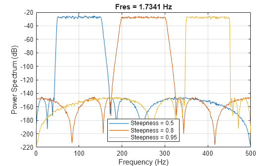
Filter white noise sampled at 1 kHz using an infinite impulse response bandpass filter with a passband width of 100 Hz. Use different steepness values. Plot the spectra of the filtered signals.
fs = 1000; x = randn(20000,1); [y1,d1] = bandpass(x,[ 50 150],fs,ImpulseResponse="iir",Steepness=0.5); [y2,d2] = bandpass(x,[200 300],fs,ImpulseResponse="iir",Steepness=0.8); [y3,d3] = bandpass(x,[350 450],fs,ImpulseResponse="iir",Steepness=0.95); pspectrum([y1 y2 y3],fs) legend("Steepness = " + [0.5 0.8 0.95],Location="south")
Compute and plot the frequency responses of the filters.
[h1,f] = freqz(d1,1024,fs); [h2,~] = freqz(d2,1024,fs); [h3,~] = freqz(d3,1024,fs); plot(f,mag2db(abs([h1 h2 h3]))) legend("Steepness = " + [0.5 0.8 0.95],Location="south") ylim([-100 10])
Make the filters asymmetric by specifying different values of steepness at the lower and higher passband frequencies.
[y1,d1] = bandpass(x,[ 50 150],fs,ImpulseResponse="iir",Steepness=[0.5 0.8]); [y2,d2] = bandpass(x,[200 300],fs,ImpulseResponse="iir",Steepness=[0.5 0.8]); [y3,d3] = bandpass(x,[350 450],fs,ImpulseResponse="iir",Steepness=[0.5 0.8]); pspectrum([y1 y2 y3],fs)
Compute and plot the frequency responses of the filters.
[h1,f] = freqz(d1,1024,fs); [h2,~] = freqz(d2,1024,fs); [h3,~] = freqz(d3,1024,fs); plot(f,mag2db(abs([h1 h2 h3]))) ylim([-100 10])
Input Arguments
x
— Input signal
vector | matrix
Input signal, specified as a vector or matrix.
Example: sin(2*pi*(0:127)/16)+randn(1,128)/100
specifies a noisy
sinusoid
Example: [2 1].*sin(2*pi*(0:127)'./[16 64])
specifies a two-channel
sinusoid.
Data Types: single
| double
Complex Number Support: Yes
wpass
— Normalized passband frequency range
two-element vector with elements in (0, 1)
Normalized passband frequency range, specified as a two-element vector with elements in the interval (0, 1).
fpass
— Passband frequency range
two-element vector with elements in (0,
fs
/2)
Passband frequency range, specified as a two-element vector with elements
in the interval (0, fs
/2).
fs
— Sample rate
positive real scalar
Sample rate, specified as a positive real scalar.
xt
— Input timetable
timetable
Input timetable. xt
must contain increasing, finite, and equally spaced
row times of type duration
in seconds.
If a timetable has missing or duplicate time points, you can fix it using the tips in Clean Timetable with Missing, Duplicate, or Nonuniform Times.
Example: timetable(seconds(0:4)',randn(5,1),randn(5,2))
contains a
single-channel random signal and a two-channel random signal, sampled at 1 Hz for 4
seconds.
Example: timetable(randn(5,1),randn(5,2),SampleRate=1)
contains a single-channel random signal and a two-channel random
signal, sampled at 1 Hz for 4 seconds.
Name-Value Arguments
Specify optional pairs of arguments as
Name1=Value1,...,NameN=ValueN
, where Name
is
the argument name and Value
is the corresponding value.
Name-value arguments must appear after other arguments, but the order of the
pairs does not matter.
Example: ImpulseResponse="iir",StopbandAttenuation=30
filters
the input using a minimum-order IIR filter that attenuates by 30 dB the frequencies
smaller than fpass(1)
and the frequencies larger than
fpass(2)
.
Before R2021a, use commas to separate each name and value, and enclose
Name
in quotes.
Example: 'ImpulseResponse','iir','StopbandAttenuation',30
filters the input using a minimum-order IIR filter that attenuates by 30 dB the
frequencies smaller than fpass(1)
and the frequencies larger than
fpass(2)
.
ImpulseResponse
— Type of impulse response
"auto"
(default) | "fir"
| "iir"
Type of impulse response of the filter, specified as "fir"
,
"iir"
, or "auto"
.
"fir"
— The function designs a minimum-order, linear-phase, finite impulse response (FIR) filter. To compensate for the delay, the function appends to the input signal N/2 zeros, where N is the filter order. The function then filters the signal and removes the first N/2 samples of the output.In this case, the input signal must be at least twice as long as the filter that meets the specifications.
"iir"
— The function designs a minimum-order infinite impulse response (IIR) filter and uses thefiltfilt
function to perform zero-phase filtering and compensate for the filter delay.If the signal is not at least three times as long as the filter that meets the specifications, the function designs a filter with smaller order and thus smaller steepness.
"auto"
— The function designs a minimum-order FIR filter if the input signal is long enough, and a minimum-order IIR filter otherwise. Specifically, the function follows these steps:Compute the minimum order that an FIR filter must have to meet the specifications. If the signal is at least twice as long as the required filter order, design and use that filter.
If the signal is not long enough, compute the minimum order that an IIR filter must have to meet the specifications. If the signal is at least three times as long as the required filter order, design and use that filter.
If the signal is not long enough, truncate the order to one-third the signal length and design an IIR filter of that order. The reduction in order comes at the expense of transition band steepness.
Filter the signal and compensate for the delay.
Steepness
— Transition band steepness
[0.85
0.85]
(default) | two-element vector with elements in the interval [0.5, 1) | scalar in the interval [0.5, 1)
Transition band steepness, specified as a scalar or two-element vector with elements in the interval [0.5, 1). As the steepness increases, the filter response approaches the ideal bandpass response, but the resulting filter length and the computational cost of the filtering operation also increase. See Bandpass Filter Steepness for more information.
StopbandAttenuation
— Filter stopband attenuation
60
(default) | positive scalar in dB
Filter stopband attenuation, specified as a positive scalar in dB.
Output Arguments
y
— Filtered signal
vector | matrix | timetable
Filtered signal, returned as a vector, a matrix, or a timetable with the same dimensions as the input.
d
— Bandpass filter
digitalFilter
object
Bandpass filter used in the filtering operation, returned as a digitalFilter
object.
Use
filter
(d,x)
to filter a signalx
usingd
. Unlikebandpass
, thefilter
function does not compensate for filter delay. You can also use thefiltfilt
andfftfilt
functions withdigitalFilter
objects.Use Filter Analyzer to visualize the filter response.
Use
designfilt
to edit or generate a digital filter based on frequency-response specifications.
More About
Bandpass Filter Steepness
The Steepness
argument controls the width of
a filter's transition regions. The lower the steepness, the wider the transition
region. The higher the steepness, the narrower the transition region.
To interpret the filter steepness, consider the following definitions:
The Nyquist frequency, fNyquist, is the highest frequency component of a signal that can be sampled at a given rate without aliasing. fNyquist is 1 (×π rad/sample) when the input signal has no time information, and
fs
/2 hertz when the input signal is a timetable or when you specify a sample rate.The lower and upper stopband frequencies of the filter, fstoplower and fstopupper, are the frequencies below which and above which the attenuation is equal to or greater than the value specified using
StopbandAttenuation
.The lower transition width of the filter, Wlower, is
fpass
lower – fstoplower, where the lower passband frequencyfpass
lower is the first element of the specifiedfpass
.The upper transition width of the filter, Wupper, is fstopupper –
fpass
upper, where the upper passband frequencyfpass
upper is the second element offpass
.Most nonideal filters also attenuate the input signal across the passband. The maximum value of this frequency-dependent attenuation is called the passband ripple. Every filter used by
bandpass
has a passband ripple of 0.1 dB.
To control the width of the transition bands, you can specify
Steepness
as either a two-element vector, [slower,supper], or a scalar.
When you specify Steepness
as a vector, the function:
Computes the lower transition width as
Wlower = (1 – slower) ×
fpass
lower.When the first element of
Steepness
is equal to 0.5, the transition width is 50% offpass
lower.As the first element of
Steepness
approaches 1, the transition width becomes progressively narrower until it reaches a minimum value of 1% offpass
lower.
Computes the upper transition width as
Wupper = (1 – supper) × (fNyquist –
fpass
upper).When the second element of
Steepness
is equal to 0.5, the transition width is 50% of (fNyquist –fpass
upper).As the second element of
Steepness
approaches 1, the transition width becomes progressively narrower until it reaches a minimum value of 1% of (fNyquist –fpass
upper).
When you specify Steepness
as a scalar, the function:
Computes Wlower and Wupper using the scalar value you specified.
Designs a symmetric filter with lower and upper transition widths equal to the smaller of Wlower and Wupper.
The default value of Steepness
is
[0.85 0.85]
.
Version History
Introduced in R2018a
See Also
Apps
Functions
MATLAB-Befehl
Sie haben auf einen Link geklickt, der diesem MATLAB-Befehl entspricht:
Führen Sie den Befehl durch Eingabe in das MATLAB-Befehlsfenster aus. Webbrowser unterstützen keine MATLAB-Befehle.
Select a Web Site
Choose a web site to get translated content where available and see local events and offers. Based on your location, we recommend that you select: .
You can also select a web site from the following list:
How to Get Best Site Performance
Select the China site (in Chinese or English) for best site performance. Other MathWorks country sites are not optimized for visits from your location.
Americas
- América Latina (Español)
- Canada (English)
- United States (English)
Europe
- Belgium (English)
- Denmark (English)
- Deutschland (Deutsch)
- España (Español)
- Finland (English)
- France (Français)
- Ireland (English)
- Italia (Italiano)
- Luxembourg (English)
- Netherlands (English)
- Norway (English)
- Österreich (Deutsch)
- Portugal (English)
- Sweden (English)
- Switzerland
- United Kingdom (English)