bandstop
Bandstop-filter signals
Syntax
Description
y = bandstop(x,wpass)x using a bandstop filter with a
stopband frequency range specified by the two-element vector
wpass and expressed in normalized units of
π rad/sample. bandstop uses a
minimum-order filter with a stopband attenuation of 60 dB and compensates for
the delay introduced by the filter. If x is a matrix, the
function filters each column independently.
y = bandstop(___,Name=Value)
[
also returns the y,d] = bandstop(___)digitalFilter object
d used to filter the input.
bandstop(___) with no output arguments plots
the input signal and overlays the filtered signal.
Examples
Create a signal sampled at 1 kHz for 1 second. The signal contains three tones, one at 50 Hz, another at 150 Hz, and a third at 250 Hz. The high-frequency and low-frequency tones both have twice the amplitude of the intermediate tone. The signal is embedded in Gaussian white noise of variance 1/100.
fs = 1e3;
t = 0:1/fs:1;
x = [2 1 2]*sin(2*pi*[50 150 250]'.*t) + randn(size(t))/10;
Bandstop-filter the signal to remove the medium-frequency tone. Specify passband frequencies of 100 Hz and 200 Hz. Display the original and filtered signals, and also their spectra.
bandstop(x,[100 200],fs)
![Figure contains 2 axes objects. Axes object 1 with title Bandstop Filtering (Fpass = [100 200] Hz), xlabel Time (s) contains 2 objects of type line. These objects represent Original, Filtered. Axes object 2 with xlabel Frequency (Hz), ylabel Power Spectrum (dB) contains 2 objects of type line. These objects represent Original, Filtered.](../../examples/signal/win64/BandstopFilteringOfTonesExample_01.png)
Implement a basic digital music synthesizer and use it to play a traditional song. Specify a sample rate of 2 kHz. Plot the spectrogram of the song.
fs = 2e3;
t = 0:1/fs:0.3-1/fs; fq = [-Inf -9:2]/12;
note = @(f,g) [1 1 1]*sin(2*pi*440*2.^[fq(g)-1 fq(g) fq(f)+1]'.*t);

mel = [5 3 1 3 5 5 5 0 3 3 3 0 5 8 8 0 5 3 1 3 5 5 5 5 3 3 5 3 1]+1;
acc = [5 0 8 0 5 0 5 5 3 0 3 3 5 0 8 8 5 0 8 0 5 5 5 0 3 3 5 0 1]+1;

song = [];
for kj = 1:length(mel)
    song = [song note(mel(kj),acc(kj)) zeros(1,0.01*fs)];
end
song = song/(max(abs(song))+0.1);

% To hear, type sound(song,fs)

pspectrum(song,fs,"spectrogram",TimeResolution=0.31, ...
    OverlapPercent=0,MinThreshold=-60)

Bandstop-filter the signal to separate the middle register from the other two. Specify passband frequencies of 230 Hz and 450 Hz. Plot the original and filtered signals in the time and frequency domains.
bong = bandstop(song,[230 450],fs);

% To hear, type sound(bong,fs)

bandstop(song,[230 450],fs)![Figure contains 2 axes objects. Axes object 1 with title Bandstop Filtering (Fpass = [230 450] Hz), xlabel Time (s) contains 2 objects of type line. These objects represent Original, Filtered. Axes object 2 with xlabel Frequency (kHz), ylabel Power Spectrum (dB) contains 2 objects of type line. These objects represent Original, Filtered.](../../examples/signal/win64/BandstopFilteringOfMusicalSignalExample_02.png)
Plot the spectrogram of the song without the middle register.
figure
pspectrum(bong,fs,"spectrogram",TimeResolution=0.31, ...
    OverlapPercent=0,MinThreshold=-60)

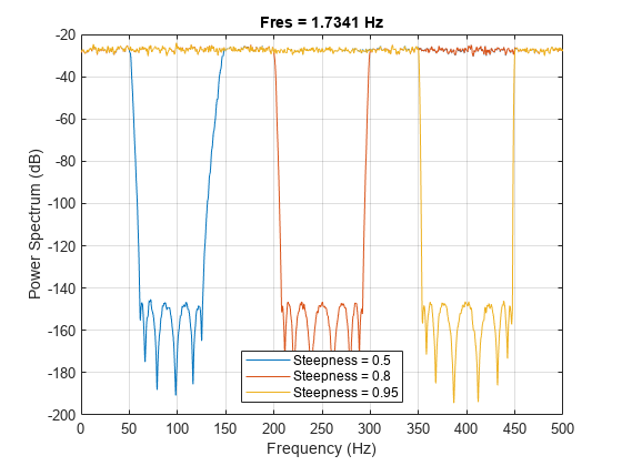
Filter white noise sampled at 1 kHz using an infinite impulse response bandstop filter with a stopband width of 100 Hz. Use different steepness values. Plot the spectra of the filtered signals.
fs = 1000;
x = randn(20000,1);

[y1,d1] = bandstop(x,[ 50 150],fs,ImpulseResponse="iir",Steepness=0.5);
[y2,d2] = bandstop(x,[200 300],fs,ImpulseResponse="iir",Steepness=0.8);
[y3,d3] = bandstop(x,[350 450],fs,ImpulseResponse="iir",Steepness=0.95);

pspectrum([y1 y2 y3],fs)
legend("Steepness = " + [0.5 0.8 0.95],Location="south")

Compute and plot the frequency responses of the filters.
[h1,f] = freqz(d1,1024,fs);
[h2,~] = freqz(d2,1024,fs);
[h3,~] = freqz(d3,1024,fs);

plot(f,mag2db(abs([h1 h2 h3])))
legend("Steepness = " + [0.5 0.8 0.95],Location="south")
ylim([-120 20])

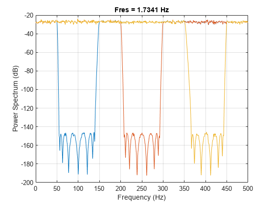
Make the filters asymmetric by specifying different values of steepness at the lower and higher passband frequencies.
[y1,d1] = bandstop(x,[ 50 150],fs,ImpulseResponse="iir",Steepness=[0.5 0.8]);
[y2,d2] = bandstop(x,[200 300],fs,ImpulseResponse="iir",Steepness=[0.5 0.8]);
[y3,d3] = bandstop(x,[350 450],fs,ImpulseResponse="iir",Steepness=[0.5 0.8]);

pspectrum([y1 y2 y3],fs)

Compute and plot the frequency responses of the filters.
[h1,f] = freqz(d1,1024,fs);
[h2,~] = freqz(d2,1024,fs);
[h3,~] = freqz(d3,1024,fs);

plot(f,mag2db(abs([h1 h2 h3])))
ylim([-120 20])

Input Arguments
Input signal, specified as a vector or matrix.
Example: sin(2*pi*(0:127)/16)+randn(1,128)/100 specifies a noisy
sinusoid
Example: [2 1].*sin(2*pi*(0:127)'./[16 64]) specifies a two-channel
sinusoid.
Data Types: single | double
Complex Number Support: Yes
Normalized stopband frequency range, specified as a two-element vector with elements in the interval (0, 1).
Stopband frequency range, specified as a two-element vector with elements
in the interval (0, fs/2).
Sample rate, specified as a positive real scalar.
Input timetable. xt must contain increasing, finite, and equally spaced
row times of type duration in seconds.
If a timetable has missing or duplicate time points, you can fix it using the tips in Clean Timetable with Missing, Duplicate, or Nonuniform Times.
Example: timetable(seconds(0:4)',randn(5,1),randn(5,2)) contains a
single-channel random signal and a two-channel random signal, sampled at 1 Hz for 4
seconds.
Example: timetable(randn(5,1),randn(5,2),SampleRate=1)
contains a single-channel random signal and a two-channel random
signal, sampled at 1 Hz for 4 seconds.
Name-Value Arguments
Specify optional pairs of arguments as
Name1=Value1,...,NameN=ValueN, where Name is
the argument name and Value is the corresponding value.
Name-value arguments must appear after other arguments, but the order of the
pairs does not matter.
Example: ImpulseResponse="iir",StopbandAttenuation=30 filters
the input using a minimum-order IIR filter that attenuates by 30 dB the frequencies
from fpass(1) to fpass(2).
Before R2021a, use commas to separate each name and value, and enclose
Name in quotes.
Example: 'ImpulseResponse','iir','StopbandAttenuation',30
filters the input using a minimum-order IIR filter that attenuates by 30 dB the
frequencies from fpass(1) to
fpass(2).
Type of impulse response of the filter, specified as "fir",
"iir", or "auto".
"fir"— The function designs a minimum-order, linear-phase, finite impulse response (FIR) filter. To compensate for the delay, the function appends to the input signal N/2 zeros, where N is the filter order. The function then filters the signal and removes the first N/2 samples of the output.In this case, the input signal must be at least twice as long as the filter that meets the specifications.
"iir"— The function designs a minimum-order infinite impulse response (IIR) filter and uses thefiltfiltfunction to perform zero-phase filtering and compensate for the filter delay.If the signal is not at least three times as long as the filter that meets the specifications, the function designs a filter with smaller order and thus smaller steepness.
"auto"— The function designs a minimum-order FIR filter if the input signal is long enough, and a minimum-order IIR filter otherwise. Specifically, the function follows these steps:Compute the minimum order that an FIR filter must have to meet the specifications. If the signal is at least twice as long as the required filter order, design and use that filter.
If the signal is not long enough, compute the minimum order that an IIR filter must have to meet the specifications. If the signal is at least three times as long as the required filter order, design and use that filter.
If the signal is not long enough, truncate the order to one-third the signal length and design an IIR filter of that order. The reduction in order comes at the expense of transition band steepness.
Filter the signal and compensate for the delay.
Transition band steepness, specified as a scalar or two-element vector with elements in the interval [0.5, 1). As the steepness increases, the filter response approaches the ideal bandstop response, but the resulting filter length and the computational cost of the filtering operation also increase. See Bandstop Filter Steepness for more information.
Filter stopband attenuation, specified as a positive scalar in dB.
Output Arguments
Filtered signal, returned as a vector, a matrix, or a timetable with the same dimensions as the input.
Bandstop filter used in the filtering operation, returned as a digitalFilter object.
Use
filter(d,x)to filter a signalxusingd. Unlikebandstop, thefilterfunction does not compensate for filter delay. You can also use thefiltfiltandfftfiltfunctions withdigitalFilterobjects.Use Filter Analyzer to visualize the filter response.
Use
designfiltto edit or generate a digital filter based on frequency-response specifications.
More About
The Steepness argument controls the width of
a filter's transition regions. The lower the steepness, the wider the transition
region. The higher the steepness, the narrower the transition region.
To interpret the filter steepness, consider the following definitions:
The Nyquist frequency, fNyquist, is the highest frequency component of a signal that can be sampled at a given rate without aliasing. fNyquist is 1 (×π rad/sample) when the input signal has no time information, and
fs/2 hertz when the input signal is a timetable or when you specify a sample rate.The lower and upper stopband frequencies of the filter, fstoplower and fstopupper, are the frequencies between which the attenuation is equal to or greater than the value specified using
StopbandAttenuation.The center of the stopband region is fcenter = (fstoplower + fstopupper)/2.
The lower transition width of the filter, Wlower, is fstoplower –
fpasslower, where the lower bandpass frequencyfpasslower is the first element of the specifiedfpass.The upper transition width of the filter, Wupper, is
fpassupper – fstopupper, where the upper bandpass frequencyfpassupper is the second element offpass.Most nonideal filters also attenuate the input signal across the passband. The maximum value of this frequency-dependent attenuation is called the passband ripple. Every filter used by
bandstophas a passband ripple of 0.1 dB.
To control the width of the transition bands, you can specify
Steepness as either a two-element vector, [slower,supper], or a scalar.
When you specify Steepness as a vector, the function:
Computes the lower transition width as
Wlower = (0.99 – 0.98slower) × (fcenter –
fpasslower).When the first element of
Steepnessis equal to 0.5, the transition width is 50% of (fcenter –fpasslower).As the first element of
Steepnessapproaches 1, the transition width becomes progressively narrower until it reaches a minimum value of 1% of (fcenter –fpasslower).
Computes the upper transition width as
Wupper = (0.99 – 0.98supper) × (
fpassupper – fcenter).When the second element of
Steepnessis equal to 0.5, the transition width is 50% of (fpassupper – fcenter).As the second element of
Steepnessapproaches 1, the transition width becomes progressively narrower until it reaches a minimum value of 1% of (fpassupper – fcenter).
When you specify Steepness as a scalar, the function:
Computes Wlower and Wupper using the scalar value you specified.
Designs a symmetric filter with lower and upper transition widths equal to the smaller of Wlower and Wupper.
The default value of Steepness is
[0.85 0.85].
Version History
Introduced in R2018a
See Also
Apps
Functions
bandpass|designfilt|filter|fir1|highpass|lowpass| Bandstop FIR | Bandstop IIR
MATLAB Command
You clicked a link that corresponds to this MATLAB command:
Run the command by entering it in the MATLAB Command Window. Web browsers do not support MATLAB commands.
Website auswählen
Wählen Sie eine Website aus, um übersetzte Inhalte (sofern verfügbar) sowie lokale Veranstaltungen und Angebote anzuzeigen. Auf der Grundlage Ihres Standorts empfehlen wir Ihnen die folgende Auswahl: .
Sie können auch eine Website aus der folgenden Liste auswählen:
So erhalten Sie die bestmögliche Leistung auf der Website
Wählen Sie für die bestmögliche Website-Leistung die Website für China (auf Chinesisch oder Englisch). Andere landesspezifische Websites von MathWorks sind für Besuche von Ihrem Standort aus nicht optimiert.
Amerika
- América Latina (Español)
- Canada (English)
- United States (English)
Europa
- Belgium (English)
- Denmark (English)
- Deutschland (Deutsch)
- España (Español)
- Finland (English)
- France (Français)
- Ireland (English)
- Italia (Italiano)
- Luxembourg (English)
- Netherlands (English)
- Norway (English)
- Österreich (Deutsch)
- Portugal (English)
- Sweden (English)
- Switzerland
- United Kingdom (English)