Model and Control Autonomous Vehicle in Offroad Scenario

Since R2024a

Step 5 of 5 in Offroad Navigation for Autonomous Haul Trucks in Open Pit Mine

• 3
• 4
• 5

This example shows how to integrate planners and controllers designed to enable a haul truck to navigate between points of interest in an open pit mine into Simulink® and Stateflow®. It visualizes navigation on a simple map or in Unreal Engine®. This example builds on the processes introduced in these examples:

1. Create Route Planner for Offroad Navigation Using Digital Elevation Data

2. Create Onramp and Terrain-Aware Global Planners for Offroad Navigation

3. Navigate Global Path Through Offroad Terrain Using Local Planner

4. Create Path Following Model Predictive Controller

Create Autonomous Planning Stack

Set up the maps and vehicle parameters using the exampleHelperCreateBehaviorModelInputs and exampleHelperPrepMPCInputs helper functions.

addpath(genpath("Helpers"),genpath("SimModels"))
exampleHelperCreateBehaviorModelInputs
exampleHelperPrepMPCInputs

Define a start location, goal location, and initial translation and rotation for the haul truck. The start location and goal locations are given in 2-D space as [x, y, theta]. The initial translation of the truck is a 3-D xyz-coordinate, adjusting for the map center and terrain elevation. The initial rotation of the truck is a 3-D rotation as [yaw, pitch, roll].

startPose = [267.5 441.5 -pi/2]; % [x,y,theta]
goalPose  = [443.5 90 -pi/6]; % [x,y,theta]
initialTranslationTruck = [(startPose(1:2)-mapSize/2) mapHeight.getMapData(startPose(1:2))-zOffset+8];
initialRotationTruck = [startPose(3) 0 0];

Open the top-level Simulink model.

model = "IntegratedBehaviorModule";
open_system(model)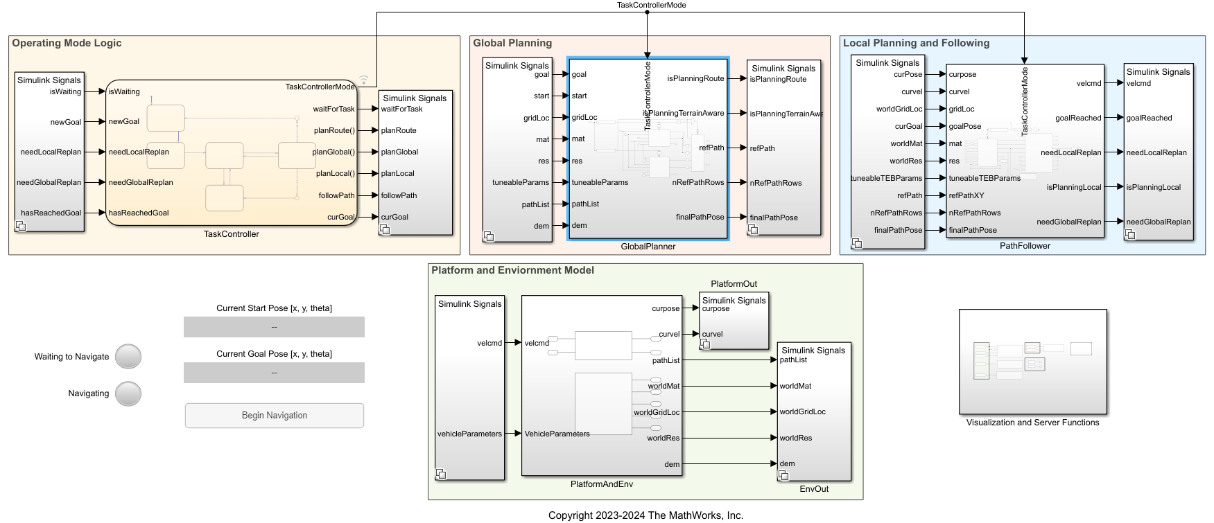

The model has five primary components:

• Operating Mode Logic — This component is the scheduler. It controls which planning algorithms are active, based on user input and the current location of the vehicle.

• Global Planning — This component includes the algorithms where the vehicle determines an overall path to get from the startPose to the goalPose. It includes the route planner developed in the Create Route Planner for Offroad Navigation Using Digital Elevation Data example, and the terrain-aware planners developed in the Create Onramp and Terrain-Aware Global Planners for Offroad Navigation example. The route planner plans along the road network and the terrain-aware planners plan in free space outside the road network.

• Local Planning — This component includes the algorithms that help the vehicle plan an obstacle-free local path along the reference path while conforming to the kinematic and geometric constraints of the haul truck. It includes the local planner developed in the Navigate Global Path Through Offroad Terrain Using Local Planner example.

• Path Following — This component includes the algorithms that help the vehicle navigate along the local paths planned in the previous component. It uses the MPC-based path follower developed in the Create Path Following Model Predictive Controller example.

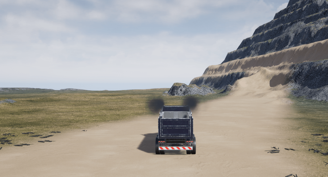
• Plant Model — This component includes the physics model for the truck, as well as information about the environment. For fast low-fidelity simulations, this component uses the bicycle kinematics model. For higher fidelity simulations, this component uses Unreal Engine®. You can specify the simulation type in the Specify Simulation Options section.

binMap = binaryOccupancyMap(~imSlope); %Define the map

Configure Simulation Options

Before running the simulation, you can configure additional options specific to the upcoming run. The exampleHelperCreateBehaviorModelInputs helper function sets default values for these parameters, but you can set them using the UI controls in this section.

Use the vssPhysModel drop-down menu to specify the platform and environment model to use for the truck.

• Simple — Use the Bicycle Kinematic Model block to represent the mining truck. Visualize the motion of the truck using the figure created in the previous section.

• Unreal — Use the Simulation 3D Physics Dump Truck block to represent the mining truck. Visualize the motion of the truck in Unreal Engine® in addition to the figure created in the previous section.

vssPhysModel = "Simple";
set_param(model + "/Plant Model", 'LabelModeActiveChoice', vssPhysModel)

Use the sliders below to change any of the vehicle's local planner parameters.

% Vehicle minimum turning radius (m)
tuneableControllerParamsCpp.MinTurningRadius = 14.2;

% Maximum-allowed linear velocity (m/s)
tuneableControllerParamsCpp.MaxVelocity(1) =16;

% Maximum-allowed angular velocity (rad/s)
tuneableControllerParamsCpp.MaxVelocity(2) =0.93;

% Maximum-allowed linear reverse velocity (m/s)
tuneableControllerParamsCpp.MaxReverseVelocity =8;

% Maximum-allowed linear acceleration (m/s^2)
tuneableControllerParamsCpp.MaxAcceleration(1) =0.6;

% Maximum-allowed angular acceleration (rad/s^2)
tuneableControllerParamsCpp.MaxAcceleration(2) =0.1;

% Safety distance between vehicle and obstacles (m)
tuneableControllerParamsCpp.ObstacleSafetyMargin = 1;

% Time steps that the controller generates velocity commands for (s)
tuneableControllerParamsCpp.LookaheadTime = 6;

Use these sliders to change the cost function optimization weights of the local planner.

% Number of Trajectories — Higher values result in a more thorough search of
% the trajectory space and potentially a better solution, at the cost of increased computations.
tuneableControllerParamsCpp.NumTrajectory =160;

% Path Following Cost — Higher values result in output trajectory trying to
% reach look ahead end pose quickly.
tuneableControllerParamsCpp.PathFollowingCost = 1;

% Path Alignment Cost — Higher values result in output trajectory trying to
% closely follow the reference path.
tuneableControllerParamsCpp.PathAlignmentCost = 1.3;

Use the drop-down menu to choose a map visualization for the simulation.

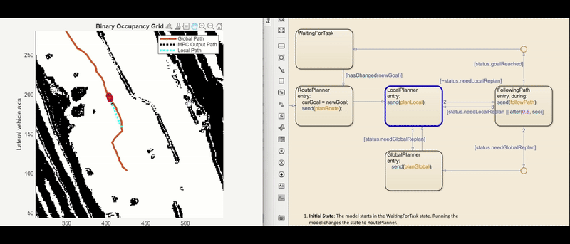
• Signed Distance Field — Map shows distances to obstacles. Points on the map return positive values if they lie outside an occupied region of space. Points on the map return negative values if they lie inside an occupied region of space. For more information about signed distance maps, see the signedDistanceMap3D (Navigation Toolbox) object.

• Binary Occupancy Map — Map shows occupied status of regions. Black cells are occupied, and white cells are unoccupied. For more information about binary occupancy maps, see the binaryOccupancyMap (Navigation Toolbox) object.

• Occupancy Map — Map shows the probability that a region is occupied. Values close to 1 (black) represent a high probability that the cell contains an obstacle. Values close to 0 (white) represent a high probability that the cell is not occupied and obstacle free. For more information about binary occupancy maps, see the occupancyMap (Navigation Toolbox) object.

maptype = 'Bin';
set_param(model + "/Visualization Functions/Map Visualization","MapType",maptype);

You can also change parameters like plotting colors, widths, and styles on the system object blocks in the Visualization Functions subsystem. By default, the map uses a binary occupancy map.

Simulate Autonomous Haul Truck

Run the model by clicking Run on the Simulation tab of the Simulink toolstrip.

You can also run the simulation programmatically by running this code.

% Start the simulation. 
sm = simulation(model);
start(sm);
% Create a figure for visualizing the map, planned paths, and the vehicle progress throughout the simulation. 
% Note that the simulation updates the figure as the simulation runs.
f = figure;
f.Visible = "on";
title("Haul Truck Simulation")
legend % Display the label for the different paths generated
pause(1);
% If the goal has been reached, end the simulation. 
pause(sm);
% Continue simulation till goalReached is false. 
while sm.SimulationOutput.logsout{1}.Values.goalReached.Data(end) == false
    t = sm.Time;
step(sm,"PauseTime",t+10); % Checks currently active state every 10 seconds of simulation time.
end

stop(sm);

Results

This example demonstrates an end-to-end offroad autonomy workflow for a haul truck using MATLAB®, Simulink, and Stateflow. A Stateflow-based scheduler coordinates global planning, local planning, and path following. The haul truck is simulated with a bicycle kinematic model and visualized on a simple 2D map and in Unreal Engine. Key parameters across the vehicle model, global planner, local planner, and controller are configurable to balance performance and fidelity. Overall, the model serves as a template for modeling, validating, and tuning autonomous haul-truck behavior in unstructured terrain.

For further information on the states in the Stateflow chart and which parts of the model they trigger, see the following table. The table also shows which of the previous examples align with each operational state.

Operational State	Subsystem	Logic/Description	Modules/Functionality	Source Example
WaitingForTask	N/A	Waits for the user to provide a new goal location. The agent reaches this state once the vehicle has reached the current goal. Setting a new goal will trigger the RoutePlanner.	N/A	N/A
RoutePlanner	GlobalPlanner/ RoutePlanner	Whenever a new goal has been assigned, the agent attempts to plan a route using RoutePlanner. This subsystem produces a reference path that is followed by the LocalPlanner and Controller subsystems.	Constructs the navGraph-based plannerAStar object. The planner then finds the nearest nodes to the current pose (curPose) and goal location (goal), and searches for the shortest path between the two. Once found, RoutePlanner uses the simple OnrampPlanner subsystem to connect curPose to the start node, and converts the sequence of edges to a dense SE2 path.	Create Route Planner for Offroad Navigation Using Digital Elevation Data
GlobalPlanner	GlobalPlanner/ TerrainAwarePlanner	In this example, the TerrainPlanner serves two primary purposes: 1) As a backup planner in the event that the LocalPlanner fails to generate a time-optimal trajectory while following the reference-path. 2) As a planner used to transition the vehicle from the end of the RoutePlanner reference-path to goal. Similar to RoutePlanner, TerrainPlanner produces a reference-path, before handing control back to LocalPlanner.	The TerrainPlanner subsystem contains the terrain-aware plannerHybridAStar module. Similar to LocalPlanner, this module takes a set of tunable parameters as input, and exposes a set of fixed mask parameters on TerrainAwarePlannerBlock.	Create Onramp and Terrain-Aware Global Planners for Offroad Navigation
LocalPlanner	LocalPlanner	This subsystem takes in the reference path produced by either the RoutePlanner or GlobalPlanner subsystems and generates a sequence of control commands which follow the reference path while avoiding local obstacles. This command sequence is forwarded to Controller, and iteratively switches between local path generation and path following until the goal has been reached or a global replan is needed.	This subsystem contains two modules: 1) A block responsible for extracting a local map from the global map. 2) A local planner variant subsystem block which can be switched between offroadControllerMPPI (default) and controllerTEB. This subsystem takes tuneableControllerParams as input, and contains additional fixed mask parameters on tebControllerBlock and mppiControllerBlock. The agent forwards time-stamped control sequences and optimized path to the FollowingPath subsystem.	Navigate Global Path Through Offroad Terrain Using Local Planner
FollowingPath	PathFollower	The Controller subsystem is tasked with producing a smooth velocity command given the local path and current time step. The controller is also responsible for determining whether a new local plan should be requested, and checks whether the vehicle has either reached the end of the reference-path, or reached the goal. If the agent has reached the end of the reference path, which corresponds to goal, then the agent returns to the WaitingForTask mode, otherwise the controller requests a global plan, which should produce a new reference path between the current location and the goal state from GlobalPlanner.	This subsystem takes in the local path from the LocalPlanner subsystem. The local path is fed to a variant subsystem, which offers two control modes: 1) LocalPlannerIndexer: Index into the optimal control sequence based on the elapsed simulation time. 2) LocalPlannerMPCCascade: Use an MPC-based controller to generate vehicle commands for the current time step. This controller uses an incoming SE2 path to generate a set of reference states for the MPC optimizer. For performance reasons, this controller only takes vehicle kinematics/constraints into account, and assumes that the provided reference path is collision free.	Create Path Following Model Predictive Controller