rlContinuousDeterministicTransitionFunction

R2026b

Deterministic transition function approximator object for neural network-based environment

Since R2022a

Description

When creating a neural network-based environment using rlNeuralNetworkEnvironment, you can specify deterministic transition function approximators using rlContinuousDeterministicTransitionFunction objects.

A transition function approximator object uses a deep neural network to predict the next observations based on the current observations and actions.

To specify stochastic transition function approximators, use rlContinuousGaussianTransitionFunction objects.

Creation

Syntax

tsnFcnAppx = rlContinuousDeterministicTransitionFunction(net,observationInfo,actionInfo,Name=Value)

Description

tsnFcnAppx = rlContinuousDeterministicTransitionFunction(net,observationInfo,actionInfo,Name=Value) creates a deterministic transition function approximator object using the deep neural network net.

When creating a deterministic transition function approximator you must specify the names of the deep neural network inputs and outputs using the ObservationInputNames, ActionInputNames, and NextObservationOutputNames name-value pair arguments.

You can also specify the PredictDiff and UseDevice properties using optional name-value pair arguments. For example, to use a GPU for prediction, specify UseDevice="gpu".

Input Arguments

net — Deep neural network

dlnetwork object

Deep neural network, specified as a dlnetwork object.

The input layer names for this network must match the input names specified using ObservationInputNames and ActionInputNames. The dimensions of the input layers must match the dimensions of the corresponding observation and action specifications in observationInfo and actionInfo, respectively.

The output layer names for this network must match the output names specified using NextObservationOutputNames. The dimensions of the output layers must match the dimensions of the corresponding observation specifications in observationInfo.

observationInfo — Observation specifications

rlNumericSpec object | array of rlNumericSpec objects

Observation specifications, specified as an rlNumericSpec object or an array of such objects. Each element in the array defines the properties of an environment observation channel, such as its dimensions, data type, and name.

This argument sets the ObservationInfo property.

Example: observationInfo=[rlNumericSpec([2 1]) rlNumericSpec([4 1])]

actionInfo — Action specifications

rlFiniteSetSpec object | rlNumericSpec object

Action specifications, specified as an rlFiniteSetSpec (for discrete action spaces) or rlNumericSpec (for continuous action spaces) object. This object defines the properties of the environment action channel, such as its dimensions, data type, and name.

This argument sets the ActionInfo property.

Example: actionInfo=rlNumericSpec([2 1])

Name-Value Arguments

Specify optional pairs of arguments as Name1=Value1,...,NameN=ValueN, where Name is the argument name and Value is the corresponding value. Name-value arguments must appear after other arguments, but the order of the pairs does not matter.

Example: ObservationInputNames="velocity"

ObservationInputNames — Observation input layer names

string | string array

Observation input layer names, specified as a string or string array.

The number of observation input names must match the length of ObservationInfo and the order of the names must match the order of the specifications in ObservationInfo.

Example: ObservationInputNames={"obsInLyr1_airspeed","obsInLyr2_altitude"}

ActionInputNames — Action input layer names

string | string array

Action input layer names, specified as a string or string array.

The number of action input names must match the length of ActionInfo and the order of the names must match the order of the specifications in ActionInfo.

Example: ActionInputNames="actInLyr_Force"

NextObservationOutputNames — Next observation output layer names

string | string array

Next observation output layer names, specified as a string or string array.

The number of next observation output names must match the length of ObservationInfo and the order of the names must match the order of the specifications in ObservationInfo.

Example: NextObservationOutputNames={"nextObsOutLyr1_airspeed","nextObsOutLyr2_altitude"}

UseDevice — Computation device used for training and simulation

"cpu" (default) | "gpu"

Computation device used for training and simulation, specified as "cpu" or "gpu". By default, the approximator uses "cpu" for training and simulation. This argument sets the UseDevice property.

Example: UseDevice="gpu"

Properties

PredictDiff — Option to predict the difference between the current observation and the next observation

false (default) | true

Option to predict the difference between the current observation and the next observation, specified as one of the following logical values.

• false — Select this option if net outputs the value of the next observation.

• true — Select this option if net outputs the difference between the next observation and the current observation. In this case, the predict function computes the next observation by adding the current observation to the output of net.

Example: PredictDiff=true

ObservationInfo — Observation specifications

Read-only: rlNumericSpec object | array of rlNumericSpec objects

This property is read-only.

Observation specifications, specified as an rlNumericSpec object or an array of such objects. Each element in the array defines the properties of an environment observation channel, such as its dimensions, data type, and name.

When you create the approximator object, the constructor function sets the ObservationInfo property to the input argument observationInfo.

You can extract observationInfo from an existing environment, function approximator, or agent using getObservationInfo. You can also construct the specifications manually using rlNumericSpec.

ActionInfo — Action specifications

Read-only: rlFiniteSetSpec object | rlNumericSpec object

This property is read-only.

Action specifications, specified either as an rlFiniteSetSpec (for discrete action spaces) or rlNumericSpec (for continuous action spaces) object. This object defines the properties of the environment action channel, such as its dimensions, data type, and name.

Note

For this approximator object, only one action channel is allowed.

When you create the approximator object, the constructor function sets the ActionInfo property to the input argument actionInfo.

You can extract ActionInfo from an existing environment or agent using getActionInfo. You can also construct the specifications manually using rlFiniteSetSpec or rlNumericSpec.

Normalization — Normalization method

"none" (default) | string array

Normalization method, returned as an array in which each element (one for each input channel defined in the observationInfo and actionInfo properties, in that order) is one of the following values:

• "none" — Do not normalize the input.

• "rescale-zero-one" — Normalize the input by rescaling it to the interval between 0 and 1. The normalized input Y is (U–Min)./(UpperLimit–LowerLimit), where U is the nonnormalized input. Note that nonnormalized input values lower than LowerLimit result in normalized values lower than 0. Similarly, nonnormalized input values higher than UpperLimit result in normalized values higher than 1. Here, UpperLimit and LowerLimit are the corresponding properties defined in the specification object of the input channel.

• "rescale-symmetric" — Normalize the input by rescaling it to the interval between –1 and 1. The normalized input Y is 2(U–LowerLimit)./(UpperLimit–LowerLimit) – 1, where U is the nonnormalized input. Note that nonnormalized input values lower than LowerLimit result in normalized values lower than –1. Similarly, nonnormalized input values higher than UpperLimit result in normalized values higher than 1. Here, UpperLimit and LowerLimit are the corresponding properties defined in the specification object of the input channel.

Note

When you specify the Normalization property of rlAgentInitializationOptions, normalization is applied only to the approximator input channels corresponding to rlNumericSpec specification objects in which both the UpperLimit and LowerLimit properties are defined. After you create the agent, you can use the setNormalizer function to assign normalizers that use any normalization method. For more information on normalizer objects, see rlNormalizer.

Example: myActor.Normalization = "rescale-symmetric" sets to "rescale-symmetric" the Normalization property of the function approximator myActor.

UseDevice — Computation device used for training and simulation

"cpu" (default) | "gpu"

Computation device used to perform operations such as gradient computation, parameter update and prediction during training and simulation, specified as either "cpu" or "gpu".

The "gpu" option requires both Parallel Computing Toolbox™ software and a CUDA^® enabled NVIDIA^® GPU. For more information on supported GPUs see GPU Computing Requirements (Parallel Computing Toolbox).

You can use gpuDevice (Parallel Computing Toolbox) to query or select a local GPU device to be used with MATLAB^®.

Note

Training or simulating an agent on a GPU involves device-specific numerical round-off errors. Because of these errors, you can get different results on a GPU and on a CPU for the same operation.

To scale up the number of environment simulations by using parallel processing over multiple cores, you do not need to use this property. Instead, set the UseParallel training option to "on" or "auto". For more information about training using multicore processors and GPUs for training, see Train Agents Using Parallel Computing and GPUs.

Example: myCritic.UseDevice = "gpu" sets to "gpu" the UseDevice property of the function approximator myCritic.

Learnables — Learnable parameters of approximator object

cell array of dlarray objects

Learnable parameters of the approximator object, specified as a cell array of dlarray objects. This property contains the learnable parameters of the approximation model used by the approximator object.

Example: myActor.Learnables = {dlarray(rand(256,4)),dlarray(rand(256,1))} sets the learnable parameters of the function approximator myActor.

State — State of approximator object

cell array of dlarray objects

State of the approximator object, specified as a cell array of dlarray objects. For dlnetwork-based models, this property contains the Value column of the State property table of the dlnetwork model. The elements of the cell array are the state of the recurrent neural network used in the approximator (if any), as well as the state for the batch normalization layer (if used).

For model types that are not based on a dlnetwork object, this property is an empty cell array, since these model types do not support states.

Example: myCritic.State={dlarray(rand(256,1)),dlarray(rand(256,1))} sets the state of the function approximator myCritic.

Object Functions

rlNeuralNetworkEnvironment

Environment model with deep neural network transition models

Examples

Create Deterministic Transition Function and Predict Next Observation

Create an environment object and extract observation and action specifications. Alternatively, you can create specifications using rlNumericSpec and rlFiniteSetSpec.

env = rlPredefinedEnv("CartPole-Continuous");
obsInfo = getObservationInfo(env);
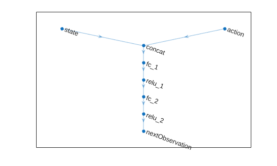
actInfo = getActionInfo(env);

To approximate the transition function, create a deep neural network. The network has two input layers, one for the current observation channel and one for the current action channel. The single output layer is for the predicted next observation.

Define each network path as an array of layer objects. Get the dimensions of the observation and action spaces from the environment specifications, and specify a name for the input and output layers, so you can later explicitly associate them with the appropriate environment channel.

statePath = featureInputLayer(obsInfo.Dimension(1),Name="state");
actionPath = featureInputLayer(actInfo.Dimension(1),Name="action");
commonPath = [
    concatenationLayer(1,2,Name="concat")
    fullyConnectedLayer(64)
    reluLayer
    fullyConnectedLayer(64)
    reluLayer
    fullyConnectedLayer(obsInfo.Dimension(1),Name="nextObservation")
    ];

Create dlnetwork object and add layers.

tsnNet = dlnetwork();
tsnNet = addLayers(tsnNet,statePath);
tsnNet = addLayers(tsnNet,actionPath);
tsnNet = addLayers(tsnNet,commonPath);

Connect layers.

tsnNet = connectLayers(tsnNet,"state","concat/in1");
tsnNet = connectLayers(tsnNet,"action","concat/in2");

Plot network.

plot(tsnNet)

Initialize network and display the number of weights.

tsnNet = initialize(tsnNet);
summary(tsnNet)

   Initialized: true

   Number of learnables: 4.8k

   Inputs:
      1   'state'    4 features
      2   'action'   1 features

Create a deterministic transition function object.

tsnFcnAppx = rlContinuousDeterministicTransitionFunction( ...
    tsnNet,obsInfo,actInfo, ...
    ObservationInputNames="state", ...
    ActionInputNames="action", ...
    NextObservationOutputNames="nextObservation");

Using this transition function object, you can predict the next observation based on the current observation and action. For example, predict the next observation for a random observation and action.

obs = rand(obsInfo.Dimension);
act = rand(actInfo.Dimension);
nextObsP = predict(tsnFcnAppx,{obs},{act})

nextObsP = 1×1 cell array
    {4×1 single}

nextObsP{1}

ans = 4×1 single column vector

   -0.1172
    0.1168
    0.0493
   -0.0155

You can also obtain the same result using evaluate.

nextObsE = evaluate(tsnFcnAppx,{obs,act})

nextObsE = 1×1 cell array
    {4×1 single}

nextObsE{1}

ans = 4×1 single column vector

   -0.1172
    0.1168
    0.0493
   -0.0155

Extended Capabilities

GPU Arrays
Accelerate code by running on a graphics processing unit (GPU) using Parallel Computing Toolbox™.

Version History

Introduced in R2022a