approximateEntropy

Measure of regularity of nonlinear time series

Syntax

approxEnt = approximateEntropy(X)

approxEnt = approximateEntropy(X,lag)

approxEnt = approximateEntropy(X,[],dim)

approxEnt = approximateEntropy(X,lag,dim)

approxEnt = approximateEntropy(___,Name,Value)

Description

approxEnt = approximateEntropy(X) estimates the approximate entropy of the uniformly sampled time-domain signal X by reconstructing the phase space. Approximate entropy is a measure to quantify the amount of regularity and unpredictability of fluctuations over a time series.

approxEnt = approximateEntropy(X,lag) estimates the approximate entropy for the time delay lag.

approxEnt = approximateEntropy(X,[],dim) estimates the approximate entropy for the embedding dimension dim.

approxEnt = approximateEntropy(X,lag,dim) estimates the approximate entropy for the time delay lag and the embedding dimension dim.

approxEnt = approximateEntropy(___,Name,Value) estimates the approximate entropy with additional options specified by one or more Name,Value pair arguments.

Examples

Compute Approximate Entropy of Signals

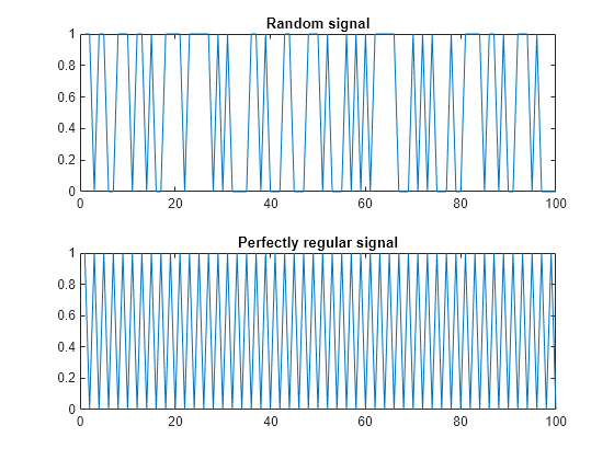
For this example, generate two signals for comparison $-$ a random signal xRand and a perfectly regular signal xReg. Set rng to default for reproducibility of the random signal.

rng('default');
xRand = double(randn(100,1)>0);
xReg = repmat([1;0],50,1);

Visualize the random and regular signals.

figure;
subplot(2,1,1);
plot(xRand);
title('Random signal');
subplot(2,1,2);
plot(xReg);
title('Perfectly regular signal');

The plots show that the regular signal is more predictable than the random signal.

Find approximate entropy of the two signals.

valueReg = approximateEntropy(xReg)

valueReg = 
5.1016e-05

valueIrreg = approximateEntropy(xRand)

valueIrreg = 
0.6849

The approximate entropy of the perfectly regular signal is significantly smaller than the random signal. Hence, the perfectly regular signal containing many repetitive patterns has a relatively small value of approximate entropy while the less predictable random signal has a higher value of approximate entropy.

Find Approximate Entropy of Data

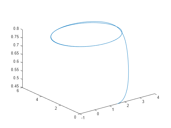
In this example, consider the position data of a quadcopter, following a circular path. The file uavPositionData.mat contains the x, y and z-direction position data traversed by the copter.

Load the data set and visualize the quadcopter path in 3D.

load('uavPositionData.mat','xv','yv','zv');
plot3(xv,yv,zv);

For this example, use only x-direction position data for computation. Since Lag is unknown, estimate the delay using phaseSpaceReconstruction. Set 'Dimension' to 3. The Dimension and Lag parameters are required to compute the approximate entropy of the data.

dim = 3;
[~,lag] = phaseSpaceReconstruction(xv,[],dim)

lag = 
4

Find the approximate entropy using the Lag value obtained in the previous step.

approxEnt = approximateEntropy(xv,lag,dim)

approxEnt = 
0.1088

Since the quadcopter is traversing a pre-defined circular trajectory of fixed radius, the position data is regular and hence, the value of approximate entropy is low.

Input Arguments

X — Uniformly sampled time-domain signal

vector | array | timetable

Uniformly sampled time-domain signal, specified as either a vector, array, or timetable. If X has multiple columns, approximateEntropy computes the approximate entropy by treating X as a multivariate signal.

If X is specified as a row vector, approximateEntropy treats it as a univariate signal.

dim — Embedding dimension

scalar | vector

Embedding dimension, specified as a scalar or vector. dim is equivalent to the 'Dimension' name-value pair.

lag — Time delay

scalar | vector

Time delay, specified as a scalar or vector. lag is equivalent to the 'Lag' name-value pair.

Name-Value Arguments

Specify optional pairs of arguments as Name1=Value1,...,NameN=ValueN, where Name is the argument name and Value is the corresponding value. Name-value arguments must appear after other arguments, but the order of the pairs does not matter.

Before R2021a, use commas to separate each name and value, and enclose Name in quotes.

Example: ...,'Dimension',3

Dimension — Embedding dimension

2 (default) | scalar | vector

Embedding dimension, specified as the comma-separated pair consisting of 'Dimension' and a scalar or vector. When Dimension is scalar, every column in X is reconstructed using Dimension. When Dimension is a vector having same length as the number of columns in X, the reconstruction dimension for column i is Dimension(i).

Specify Dimension based on the dimension of your system. For more information on embedding dimension, see phaseSpaceReconstruction.

Lag — Delay in phase space reconstruction

1 (default) | scalar | vector

Delay in phase space reconstruction, specified as the comma-separated pair consisting of 'Lag' and a scalar. When Lag is scalar, every column in X is reconstructed using Lag. When Lag is a vector having same length as the number of columns in X, the reconstruction delay for column i is Lag(i).

If the delay is too small, random noise is introduced in the data. In contrast, if the lag is too large, the reconstructed dynamics does not represent the true dynamics of the time series. For more information on calculating optimal delay, see phaseSpaceReconstruction.

Radius — Similarity criterion

0.2*std(X) | 0.2*sqrt(trace(cov(X))) | scalar

Similarity criterion, specified as the comma-separated pair consisting of 'Radius' and a scalar. The similarity criterion, also called radius of similarity, is a tuning parameter that is used to identify a meaningful range in which fluctuations in data are to be considered similar.

The default value of Radius is,

• 0.2*std(X), if X has a single column.

• 0.2*sqrt(trace(cov(X))), if X has multiple columns.

Output Arguments

approxEnt — Approximate entropy of nonlinear time series

scalar

Approximate entropy of nonlinear time series, returned as a scalar. Approximate entropy is a regularity statistic that quantifies the unpredictability of fluctuations in a time series. A relatively higher value of approximate entropy reflects the likelihood that similar patterns of observations are not followed by additional similar observations.

For example, consider two binary signals S1 and S2,

S1 = [0 1 0 1 0 1 0 1 0 1 0 1 0 1 0 1];

S2 = [1 1 0 1 1 1 1 0 1 0 1 0 0 0 0 1];

Signal S1 is perfectly regular since it alternates between 0 and 1, that is, you can predict the next value with knowledge of the previous value. Signal S2 however offers no insight into the next value, even with prior knowledge of the previous value. Hence, signal S2 is random and less predictable. Therefore, a signal containing highly repetitive patterns has a relatively small value of approxEnt while a less predictable signal has a relatively larger value of approxEnt.

Use approximateEntropy as a measure of regularity to quantify levels of complexity within a time series. The ability to discern levels of complexity within data sets is useful in the field of engineering to estimate component failure by studying their vibration and acoustic signals, or in the clinical domain where, for instance, the chance of a seizure is predicted by observing Electroencephalography (EEG) patterns.[2][3]

Algorithms

Approximate entropy is computed in the following way,

1. The approximateEntropy function first generates a delayed reconstruction Y_1:N for N data points with embedding dimension m, and lag τ.

2. The software then calculates the number of within range points, at point i, given by,

   $$N_i={\displaystyle \sum _{i=1,i\ne k}^{N}1\left({\Vert Y_i-Y_k\Vert }_{\infty }<R\right)}$$

   where 1 is the indicator function, and R is the radius of similarity.

3. The approximate entropy is then calculated as $$approxEnt={\Phi }_m-{\Phi }_{m+1}$$ where,

   $${\Phi }_m={\left(N-m+1\right)}^{-1}{\displaystyle \sum _{i=1}^{N-m+1}\log \left(N_i\right)}$$

References

[1] Pincus, Steven M. "Approximate entropy as a measure of system complexity." Proceedings of the National Academy of Sciences. 1991 88 (6) 2297-2301; doi:10.1073/pnas.88.6.2297.

[2] U. Rajendra Acharya, Filippo Molinari, S. Vinitha Sree, Subhagata Chattopadhyay, Kwan-Hoong Ng, Jasjit S. Suri. "Automated diagnosis of epileptic EEG using entropies." Biomedical Signal Processing and Control Volume 7, Issue 4, 2012, Pages 401-408, ISSN 1746-8094.

[3] Caesarendra, Wahyu & Kosasih, P & Tieu, Kiet & Moodie, Craig. "An application of nonlinear feature extraction-A case study for low speed slewing bearing condition monitoring and prognosis." IEEE/ASME International Conference on Advanced Intelligent Mechatronics: Mechatronics for Human Wellbeing, AIM 2013.1713-1718. 10.1109/AIM.2013.6584344.

[4] Kantz, H., and Schreiber, T. Nonlinear Time Series Analysis. Cambridge: Cambridge University Press, 2003.

Extended Capabilities

C/C++ Code Generation
Generate C and C++ code using MATLAB® Coder™.

Version History

Introduced in R2018a