Main Content

rsample

Random sampling of linear identified systems

Syntax

sys_array = rsample(sys,N)
sys_array = rsample(sys,N,sd)

Description

sys_array = rsample(sys,N) creates N random samples of the identified linear system, sys. sys_array contains systems with the same structure as sys, whose parameters are perturbed about their nominal values, based on the parameter covariance.

sys_array = rsample(sys,N,sd) specifies the standard deviation level, sd, for perturbing the parameters of sys.

Input Arguments

sys

Identifiable system.

N

Number of samples to be generated.

Default: 10

sd

Standard deviation level for perturbing the identifiable parameters of sys.

Default: 1

Output Arguments

sys_array

Array of random samples of sys.

If sys is an array of models, then the size of sys_array is equal to [size(sys) N]. There are N randomized samples for each model in sys.

The parameters of the samples in sys_array vary from the original identifiable model within 1 standard deviation of their nominal values.

Examples

collapse all

Estimate a third-order, discrete-time, state-space model.

load iddata2 z2;
sys = n4sid(z2,3);

Randomly sample the estimated model.

N = 20;
sys_array = rsample(sys,N);

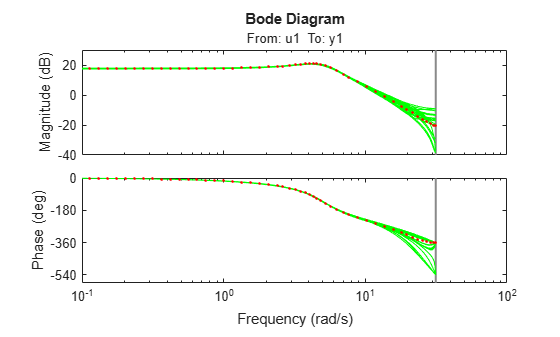
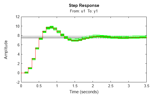
Analyze the uncertainty in time (step) and frequency (Bode) responses.

opt = bodeoptions;
opt.PhaseMatching = 'on';
figure;
bodeplot(sys_array,'g',sys,'r.',opt)

Figure contains 2 axes objects. Axes object 1 with title From: u1 To: y1, ylabel Magnitude (dB) contains 21 objects of type line. One or more of the lines displays its values using only markers These objects represent sys\_array, sys. Axes object 2 with ylabel Phase (deg) contains 21 objects of type line. One or more of the lines displays its values using only markers These objects represent sys\_array, sys.

figure;
stepplot(sys_array,'g',sys,'r.-')

Figure contains an axes object. The axes object with title From: u1 To: y1 contains 21 objects of type line. These objects represent sys\_array, sys.

Estimate a third-order, discrete-time, state-space model.

load iddata2 z2;
sys = n4sid(z2,3);

Randomly sample the estimated model. Specify the standard deviation level for perturbing the model parameters.

N = 20;
sd = 2;
sys_array = rsample(sys,N,sd);

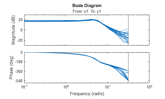
Analyze the model uncertainty.

figure;
bode(sys_array);

Figure contains 2 axes objects. Axes object 1 with title From: u1 To: y1, ylabel Magnitude (dB) contains 20 objects of type line. This object represents sys\_array. Axes object 2 with ylabel Phase (deg) contains 20 objects of type line. This object represents sys\_array.

Estimate an ARMAX model.

load iddata1 z1
sys = armax(z1,[2 2 2 1]);

Randomly sample the ARMAX model. Perturb the model parameters up to 2 standard deviations.

N = 20;
sd = 2;
sys_array = rsample(sys,N,sd);

Compare the frequency response confidence region corresponding to 2 standard deviations (asymptotic estimate) with the model array response.

opt = bodeoptions; opt.PhaseMatching = 'on';
opt.ConfidenceRegionNumberSD = 2;
bodeplot(sys_array,'g',sys,'r',opt)

Figure contains 2 axes objects. Axes object 1 with title From: u1 To: y1, ylabel Magnitude (dB) contains 21 objects of type line. These objects represent sys\_array, sys. Axes object 2 with ylabel Phase (deg) contains 21 objects of type line. These objects represent sys\_array, sys.

To view the confidence region, right click the plot, and choose Characteristics > Confidence Region.

Tips

  • For systems with large parameter uncertainties, the randomized systems may contain unstable elements. These unstable elements may make it difficult to analyze the properties of the identified system. Execution of analysis commands, such as step, bode, sim, etc., on such systems can produce unreliable results. Instead, use a dedicated Monte-Carlo analysis command, such as simsd.

Version History

Introduced in R2012a