ahrsfilter
Orientation from accelerometer, gyroscope, and magnetometer readings
Description
The ahrsfilter
System object™ fuses accelerometer, magnetometer, and gyroscope sensor data to estimate device
orientation.
To estimate device orientation:
Create the
ahrsfilterobject and set its properties.Call the object with arguments, as if it were a function.
To learn more about how System objects work, see What Are System Objects?
Creation
Description
FUSE = ahrsfilterFUSE, for sensor fusion of accelerometer, gyroscope, and
magnetometer data to estimate device orientation and angular velocity. The filter uses a
12-element state vector to track the estimation error for the orientation, the gyroscope
bias, the linear acceleration, and the magnetic disturbance.
FUSE = ahrsfilter('ReferenceFrame',RF)ahrsfilter
System object that fuses accelerometer, gyroscope, and magnetometer data to estimate
device orientation relative to the reference frame RF.
FUSE = ahrsfilter(___,Name=Value)
Input Arguments
Properties
Usage
Description
[
fuses accelerometer, gyroscope, and magnetometer data to compute orientation and angular
velocity measurements. The algorithm assumes that the device is stationary before the
first call.orientation,angularVelocity,interData] = FUSE(accelReadings,gyroReadings,magReadings)
Input Arguments
Output Arguments
Object Functions
To use an object function, specify the
System object as the first input argument. For
example, to release system resources of a System object named obj, use
this syntax:
release(obj)
Examples
Load the rpy_9axis file, which contains recorded accelerometer, gyroscope, and magnetometer sensor data from a device oscillating in pitch (around y-axis), then yaw (around z-axis), and then roll (around x-axis). The file also contains the sample rate of the recording.
load 'rpy_9axis' sensorData Fs
accelerometerReadings = sensorData.Acceleration;
gyroscopeReadings = sensorData.AngularVelocity;
magnetometerReadings = sensorData.MagneticField;
Create an ahrsfilter System object™ with SampleRate set to the sample rate of the sensor data. Specify a decimation factor of two to reduce the computational cost of the algorithm.
decim = 2;
fuse = ahrsfilter('SampleRate',Fs,'DecimationFactor',decim);
Pass the accelerometer readings, gyroscope readings, and magnetometer readings to the ahrsfilter object, fuse, to output an estimate of the sensor body orientation over time. By default, the orientation is output as a vector of quaternions.
q = fuse(accelerometerReadings,gyroscopeReadings,magnetometerReadings);
Orientation is defined by angular displacement required to rotate a parent coordinate system to a child coordinate system. Plot the orientation in Euler angles in degrees over time.
ahrsfilter correctly estimates the change in orientation over time, including the south-facing initial orientation.
time = (0:decim:size(accelerometerReadings,1)-1)/Fs;

plot(time,eulerd(q,'ZYX','frame'))
title('Orientation Estimate')
legend('z-axis', 'y-axis', 'x-axis')
ylabel('Rotation (degrees)')

This example shows how performance of the ahrsfilter System object™ is affected by magnetic jamming.
Load StationaryIMUReadings, which contains accelerometer, magnetometer, and gyroscope readings from a stationary IMU.
load 'StationaryIMUReadings.mat' accelReadings magReadings gyroReadings SampleRate

numSamples = size(accelReadings,1);
The ahrsfilter uses magnetic field strength to stabilize its orientation against the assumed constant magnetic field of the Earth. However, there are many natural and man-made objects which output magnetic fields and can confuse the algorithm. To account for the presence of transient magnetic fields, you can set the MagneticDisturbanceNoise property on the ahrsfilter object.
Create an ahrsfilter object with the decimation factor set to 2 and note the default expected magnetic field strength.
decim = 2;
FUSE = ahrsfilter('SampleRate',SampleRate,'DecimationFactor',decim);
Fuse the IMU readings using the attitude and heading reference system (AHRS) filter, and then visualize the orientation of the sensor body over time. The orientation fluctuates at the beginning and stabilizes after approximately 60 seconds.
orientation = FUSE(accelReadings,gyroReadings,magReadings);

orientationEulerAngles = eulerd(orientation,'ZYX','frame');
time = (0:decim:(numSamples-1))'/SampleRate;

figure(1)
plot(time,orientationEulerAngles(:,1), ...
     time,orientationEulerAngles(:,2), ...
     time,orientationEulerAngles(:,3))
xlabel('Time (s)')
ylabel('Rotation (degrees)')
legend('z-axis','y-axis','x-axis')
title('Filtered IMU Data')

Mimic magnetic jamming by adding a transient, strong magnetic field to the magnetic field recorded in the magReadings. Visualize the magnetic field jamming.
jamStrength = [10,5,2];
startStop = (50*SampleRate):(150*SampleRate);
jam = zeros(size(magReadings));
jam(startStop,:) = jamStrength.*ones(numel(startStop),3);

magReadings = magReadings + jam;

figure(2)
plot(time,magReadings(1:decim:end,:))
xlabel('Time (s)')
ylabel('Magnetic Field Strength (\mu T)')
title('Simulated Magnetic Field with Jamming')
legend('z-axis','y-axis','x-axis')


Run the simulation again using the magReadings with magnetic jamming. Plot the results and note the decreased performance in orientation estimation.
reset(FUSE)
orientation = FUSE(accelReadings,gyroReadings,magReadings);

orientationEulerAngles = eulerd(orientation,'ZYX','frame');

figure(3)
plot(time,orientationEulerAngles(:,1), ...
     time,orientationEulerAngles(:,2), ...
     time,orientationEulerAngles(:,3))
xlabel('Time (s)')
ylabel('Rotation (degrees)')
legend('z-axis','y-axis','x-axis')
title('Filtered IMU Data with Magnetic Disturbance and Default Properties')


The magnetic jamming was misinterpreted by the AHRS filter, and the sensor body orientation was incorrectly estimated. You can compensate for jamming by increasing the MagneticDisturbanceNoise property. Increasing the MagneticDisturbanceNoise property increases the assumed noise range for magnetic disturbance, and the entire magnetometer signal is weighted less in the underlying fusion algorithm of ahrsfilter.
Set the MagneticDisturbanceNoise to 200 and run the simulation again.
The orientation estimation output from ahrsfilter is more accurate and less affected by the magnetic transient. However, because the magnetometer signal is weighted less in the underlying fusion algorithm, the algorithm may take more time to restabilize.
reset(FUSE)
FUSE.MagneticDisturbanceNoise = 20;

orientation = FUSE(accelReadings,gyroReadings,magReadings);

orientationEulerAngles = eulerd(orientation,'ZYX','frame');

figure(4)
plot(time,orientationEulerAngles(:,1), ...
     time,orientationEulerAngles(:,2), ...
     time,orientationEulerAngles(:,3))
xlabel('Time (s)')
ylabel('Rotation (degrees)')
legend('z-axis','y-axis','x-axis')
title('Filtered IMU Data with Magnetic Disturbance and Modified Properties')

This example uses the ahrsfilter System object™ to fuse 9-axis IMU data from a sensor body that is shaken. Plot the quaternion distance between the object and its final resting position to visualize performance and how quickly the filter converges to the correct resting position. Then tune parameters of the ahrsfilter so that the filter converges more quickly to the ground-truth resting position.
Load IMUReadingsShaken into your current workspace. This data was recorded from an IMU that was shaken then laid in a resting position. Visualize the acceleration, magnetic field, and angular velocity as recorded by the sensors.
load 'IMUReadingsShaken' accelReadings gyroReadings magReadings SampleRate
numSamples = size(accelReadings,1);
time = (0:(numSamples-1))'/SampleRate;

figure(1)
subplot(3,1,1)
plot(time,accelReadings)
title('Accelerometer Reading')
ylabel('Acceleration (m/s^2)')

subplot(3,1,2)
plot(time,magReadings)
title('Magnetometer Reading')
ylabel('Magnetic Field (\muT)')

subplot(3,1,3)
plot(time,gyroReadings)
title('Gyroscope Reading')
ylabel('Angular Velocity (rad/s)')
xlabel('Time (s)')

Create an ahrsfilter and then fuse the IMU data to determine orientation. The orientation is returned as a vector of quaternions; convert the quaternions to Euler angles in degrees. Visualize the orientation of the sensor body over time by plotting the Euler angles required, at each time step, to rotate the global coordinate system to the sensor body coordinate system.
fuse = ahrsfilter('SampleRate',SampleRate);
orientation = fuse(accelReadings,gyroReadings,magReadings);

orientationEulerAngles = eulerd(orientation,'ZYX','frame');

figure(2)
plot(time,orientationEulerAngles(:,1), ...
     time,orientationEulerAngles(:,2), ...
     time,orientationEulerAngles(:,3))
xlabel('Time (s)')
ylabel('Rotation (degrees)')
title('Orientation over Time')
legend('Rotation around z-axis', ...
       'Rotation around y-axis', ...
       'Rotation around x-axis')

In the IMU recording, the shaking stops after approximately six seconds. Determine the resting orientation so that you can characterize how fast the ahrsfilter converges.
To determine the resting orientation, calculate the averages of the magnetic field and acceleration for the final four seconds and then use the ecompass function to fuse the data.
Visualize the quaternion distance from the resting position over time.
restingOrientation = ecompass(mean(accelReadings(6*SampleRate:end,:)), ...
                              mean(magReadings(6*SampleRate:end,:)));

figure(3)
plot(time,rad2deg(dist(restingOrientation,orientation)))
hold on
xlabel('Time (s)')
ylabel('Quaternion Distance (degrees)')


Modify the default ahrsfilter properties so that the filter converges to gravity more quickly. Increase the GyroscopeDriftNoise to 1e-2 and decrease the LinearAccelerationNoise to 1e-4. This instructs the ahrsfilter algorithm to weigh gyroscope data less and accelerometer data more. Because the accelerometer data provides the stabilizing and consistent gravity vector, the resulting orientation converges more quickly.
Reset the filter, fuse the data, and plot the results.
fuse.LinearAccelerationNoise = 1e-4;
fuse.GyroscopeDriftNoise     = 1e-2;
reset(fuse)

orientation = fuse(accelReadings,gyroReadings,magReadings);

figure(3)
plot(time,rad2deg(dist(restingOrientation,orientation)))
legend('Default AHRS Filter','Tuned AHRS Filter')

Algorithms
Note: The following algorithm only applies to an NED reference frame.
The ahrsfilter uses the nine-axis Kalman filter structure described in
[1]. The algorithm attempts to track the
errors in orientation, gyroscope offset, linear acceleration, and magnetic disturbance to
output the final orientation and angular velocity. Instead of tracking the orientation
directly, the indirect Kalman filter models the error process, x, with a
recursive update:
where xk is a 12-by-1 vector consisting of:
θk –– 3-by-1 orientation error vector, in degrees, at time k
bk –– 3-by-1 gyroscope zero angular rate bias vector, in deg/s, at time k
ak –– 3-by-1 acceleration error vector measured in the sensor frame, in g, at time k
dk –– 3-by-1 magnetic disturbance error vector measured in the sensor frame, in µT, at time k
and where wk is a 12-by-1 additive noise vector, and Fk is the state transition model.
Because xk is defined as the error process, the a priori estimate is always zero, and therefore the state transition model, Fk, is zero. This insight results in the following reduction of the standard Kalman equations:
Standard Kalman equations:
Kalman equations used in this algorithm:
where:
xk− –– predicted (a priori) state estimate; the error process
Pk− –– predicted (a priori) estimate covariance
yk –– innovation
Sk –– innovation covariance
Kk –– Kalman gain
xk+ –– updated (a posteriori) state estimate
Pk+ –– updated (a posteriori) estimate covariance
k represents the iteration, the superscript + represents an a posteriori estimate, and the superscript − represents an a priori estimate.
The graphic and following steps describe a single frame-based iteration through the algorithm.

Before the first iteration, the accelReadings,
gyroReadings, and magReadings inputs are chunked
into DecimationFactor-by-3 frames. For each chunk, the algorithm uses the
most current accelerometer and magnetometer readings corresponding to the chunk of gyroscope
readings.
Walk through the algorithm for an explanation of each stage of the detailed overview.
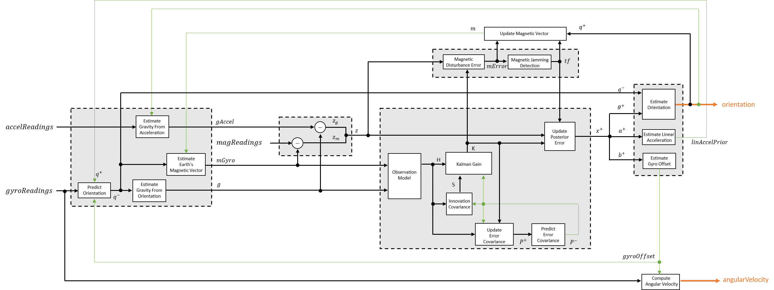
The algorithm models acceleration and angular change as linear processes.

The orientation for the current frame is predicted by first estimating the angular change from the previous frame:
where N is the decimation factor specified by the DecimationFactor property and fs is the sample rate specified by the SampleRate property.
The angular change is converted into quaternions using the rotvec
quaternion
construction syntax:
The previous orientation estimate is updated by rotating it by ΔQ:
During the first iteration, the orientation estimate,
q−, is initialized by ecompass.
The gravity vector is interpreted as the third column of the quaternion, q−, in rotation matrix form:
See [1] for an explanation of why the third column of rPrior can be interpreted as the gravity vector.
A second gravity vector estimation is made by subtracting the decayed linear acceleration estimate of the previous iteration from the accelerometer readings:
Earth's magnetic vector is estimated by rotating the magnetic vector estimate from the previous iteration by the a priori orientation estimate, in rotation matrix form:

The error model combines two differences:
The difference between the gravity estimate from the accelerometer readings and the gravity estimate from the gyroscope readings:
The difference between the magnetic vector estimate from the gyroscope readings and the magnetic vector estimate from the magnetometer:
The magnetometer correct estimates the error in the magnetic vector estimate and detects magnetic jamming.
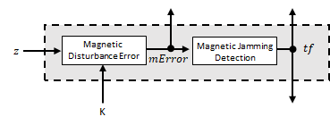
The magnetic disturbance error is calculated by matrix multiplication of the Kalman gain associated with the magnetic vector with the error signal:
The Kalman gain, K, is the Kalman gain calculated in the current iteration.
Magnetic jamming is determined by verifying that the power of the detected magnetic disturbance is less than or equal to four times the power of the expected magnetic field strength:
ExpectedMagneticFieldStrength
is a property of ahrsfilter.
The Kalman equations use the gravity estimate derived from the gyroscope readings, g, the magnetic vector estimate derived from the gyroscope readings, mGyro, and the observation of the error process, z, to update the Kalman gain and intermediary covariance matrices. The Kalman gain is applied to the error signal, z, to output an a posteriori error estimate, x+.
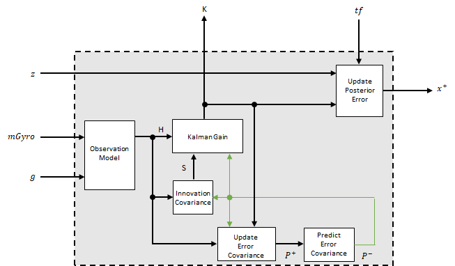
The observation model maps the 1-by-3 observed states, g and mGyro, into the 6-by-12 true state, H.
The observation model is constructed as:
where gx,
gy, and
gz are the x-,
y-, and z-elements of the gravity vector estimated
from the a priori orientation, respectively.
mx,
my, and
mz are the x-,
y-, and z-elements of the magnetic vector
estimated from the a priori orientation, respectively.
κ is a constant determined by the SampleRate
and DecimationFactor
properties: κ =
DecimationFactor/SampleRate.
See sections 7.3 and 7.4 of [1] for a derivation of the observation model.
The innovation covariance is a 6-by-6 matrix used to track the variability in the measurements. The innovation covariance matrix is calculated as:
where
H is the observation model matrix
P− is the predicted (a priori) estimate of the covariance of the observation model calculated in the previous iteration
R is the covariance of the observation model noise, calculated as:
where
and
The following properties define the observation model noise variance:
The error estimate covariance is a 12-by-12 matrix used to track the variability in the state.
The error estimate covariance matrix is updated as:
where K is the Kalman gain, H is the measurement matrix, and P− is the error estimate covariance calculated during the previous iteration.
The error estimate covariance is a 12-by-12 matrix used to track the variability in the state. The a priori error estimate covariance, P−, is set to the process noise covariance, Q, determined during the previous iteration. Q is calculated as a function of the a posteriori error estimate covariance, P+. When calculating Q, it is assumed that the cross-correlation terms are negligible compared to the autocorrelation terms, and are set to zero:
where
P+ –– is the updated (a posteriori) error estimate covariance
β –– GyroscopeDriftNoise
η –– GyroscopeNoise
See section 10.1 of [1] for a derivation of the terms of the process error matrix.
The Kalman gain matrix is a 12-by-6 matrix used to weight the innovation. In this algorithm, the innovation is interpreted as the error process, z.
The Kalman gain matrix is constructed as:
where
P− –– predicted error covariance
H –– observation model
S –– innovation covariance
The a posterior error estimate is determined by combining the Kalman gain matrix with the error in the gravity vector and magnetic vector estimations:
If magnetic jamming is detected in the current iteration, the magnetic vector error signal is ignored, and the a posterior error estimate is calculated as:

The orientation estimate is updated by multiplying the previous estimation by the error:
The linear acceleration estimation is updated by decaying the linear acceleration estimation from the previous iteration and subtracting the error:
where
The gyroscope offset estimation is updated by subtracting the gyroscope offset error from the gyroscope offset from the previous iteration:
References
[1] Open Source Sensor Fusion. https://github.com/memsindustrygroup/Open-Source-Sensor-Fusion/tree/master/docs
[2] Roetenberg, D., H.J. Luinge, C.T.M. Baten, and P.H. Veltink. "Compensation of Magnetic Disturbances Improves Inertial and Magnetic Sensing of Human Body Segment Orientation." IEEE Transactions on Neural Systems and Rehabilitation Engineering. Vol. 13. Issue 3, 2005, pp. 395-405.
Extended Capabilities
Version History
Introduced in R2018bSee Also
ecompass | imufilter | imuSensor | gpsSensor | quaternion